What’s logical coherence for anyway?

Time for a writeup! Or something.

So I’ve written before about Logical Uncertainty in a very vague way. And a few weeks ago I wrote about a specific problem of Logical Uncertainty which was presented in the MIRI workshop. I’m gonna reference definitions and results from that post here, too, though I’ll redefine:

Definition 1 (Coherence). A distribution $\mathbb P$ over a set of sentences is coherent if:

Normalisation: $\mathbb P(\top) = 1$
Additivity: $\forall \varphi,\psi:\mathbb P(\varphi) = \mathbb P(\varphi\land\psi)+\mathbb P(\varphi\land\neg\psi)$
Non-negativity: $\forall\varphi:\mathbb P(\varphi)\geq 0$
Consistency: $\forall\varphi,\psi:\varphi\equiv\psi\rightarrow\mathbb P(\varphi) = \mathbb P(\psi)$

The $\top$ symbol stands for a tautology (e.g. $0 = 0$ ), and if $\bot$ stands for a contradiction (e.g. $0 = 1$ ) then normalisation and additivity imply $\mathbb P(\bot) = 0$ , and the whole definition implies $\forall\varphi:0\leq \mathbb P(\varphi) \leq 1$ .

TL;DR: A distribution $\mathbb P$ is coherent if it’s an actual probability distribution and obeys the basic laws of probability (to perform inference you’d define $\mathbb P(\varphi|\psi) = \frac{\mathbb P(\varphi\land\psi)}{\mathbb P(\psi)}$ ).

Proposition 1. Any coherent distribution $\mathbb P$ over the set of all first-order logical sentences is uncomputable.

Proof. In first-order logic, as the Completeness Theorem says, all true statements are provable, and soundness of the first-order logic axioms means all provable statements are true. Ergo, a coherent distribution over the set of all logical sentences is Gaifman, since all true $\Pi_1$ sentences $\varphi$ are provable and therefore must have $\mathbb P(\varphi) = 1$ , as per Normalisation. Now suppose this distribution was computable. That would imply it’s also computably approximable: just take the function $f('\varphi', n) = f('\varphi') + \frac 1 {n }$ where $f('\varphi')$ is the computable function that outputs $\mathbb P(\varphi)$ . But then, this would mean that $\mathbb P$ is coherent, Gaifman, and computably approximable, and according to Theorem 1 of that post it would give probability $0$ to some true, provable $\Pi_2$ sentences, violating Normalisation: contradiction. □

I think this would probably be doubly true for second-order logical sentences, but I haven’t thought about this enough to come up with a proof. Anyway, so much for that. Let’s define something else, then:

Definition 2 (Trivial equivalence). We define a relation $\sim$ as the minimal equivalence relation satisfying the following for all sentences $\varphi$ , $\psi$ , and $\xi$ :

$(\varphi \land\psi) \sim (\psi \land \varphi)$
$(\varphi \land(\psi\land\xi)) \sim ((\varphi \land \psi)\land\xi)$
$(\varphi \land\varphi) \sim \varphi$
$(\varphi\land\neg\varphi)\sim\bot$
$(\neg\neg\varphi)\sim\varphi$
$(\varphi\land\bot)\sim\bot$
$(\varphi \land\top) \sim \varphi$
$\neg\bot\sim\top$
$(\varphi\lor\psi)\sim\neg(\neg\varphi\land\neg\psi)$
$(\varphi\rightarrow\psi)\sim(\neg\varphi\lor\psi)$
$\exists x:\varphi(x)\sim\neg\forall x:\neg\varphi(x)$

And such that, whenever $\varphi\sim\psi$ :

$\neg\varphi\sim\neg\psi$
$(\forall x:\varphi)\sim(\forall x:\psi)$
$(\varphi\land\xi)\sim(\psi\land\xi)$

Two sentences linked to each other by this relation are said to be trivially equivalent.

Paul Christiano proves that for any sentences $\varphi$ and $\psi$ you can determine whether $\varphi\sim\psi$ in $O(n\log^2n)$ time where $n$ is the total length of these sentences, which obviates the usefulness of this definition as opposed to fully general logical equivalence, which is computationally intractable.

And with that we have another definition:

Definition 3 (Local Coherence). Given a finite set of sentences $S$ , we say that a distribution $\mathbb P$ defined on that set is locally coherent if:

Weak normalisation: for all sentences $\varphi$ that are axioms or have been proven to be true, $\mathbb P(\varphi) = 1$
Additivity: $\forall \varphi,\psi \in S:\mathbb P(\varphi) = \mathbb P(\varphi\land\psi)+\mathbb P(\varphi\land\neg\psi)$
Non-negativity: $\forall\varphi\in S:\mathbb P(\varphi)\geq 0$
Weak consistency: $\forall\varphi,\psi\in S:\varphi\sim\psi\rightarrow\mathbb P(\varphi) = \mathbb P(\psi)$

This is clearly a strict weakening of the notion of coherence, and might be better to characterise realistic deductively limited logical uncertainty. Before we know that two sentences are logically equivalent, or that one implies the other, it may very well be the case that they have probabilities that aren’t coherent. However, if we could guarantee local coherence, i.e. that the things we actually know/have proven constrain our distribution, then that’d be ideal.

Let’s talk about some more of the actual workshop.

On the first day we went over the basics: what MIRI’s project is, why we care about Logical Uncertainty, and what interesting and/or open questions were. In specific, Patrick LaVictoire was talking about a certain hierarchy of constructions:

Philosophical question $\rightarrow$ Infinite computing power $\rightarrow$ Computable but intractable models $\rightarrow$ P-time models $\rightarrow$ Actually usable algorithms

The question at hand is “How do we deal with uncertainty about the output of deterministic algorithms?” And of course, if you have infinite computing power, there’s not much of a question of the matter: you just know all your (at least first-order) theorems, the end. It only really becomes interesting/hard when we get to the non-omniscient finite deductively-limited case.

Interesting questions, topics, and results about this are:

Probabilistic reflection principles
Polynomial-time approximate Bayesian updating via Kullback-Leibler divergence
Benford’s test and irreducible patterns
Asymptotic logical uncertainty
Optimal predictors (complexity theory approach)
The $\Pi_1-\Pi_2$ problem
Probability-based UDT
Reflective oracles and logical uncertainty
Integrating logical and physical uncertainty
Comparing priors
Relaxations of coherence
Noninformative (incoherent) priors

Index

1. Probabilistic reflection principles

In the Definability of Truth draft, a few interesting things are derived about probability distributions over logical sentences.

One of the things it’d be nice for any theory with a probability function over itself to have is a way of actually talking about this probability function. So, in addition to the actual distribution $\mathbb P$ , our theory will have a function symbol $P$ that refers to this distribution.

A desirable thing our distribution could have would be a sort of reflection principle:

$(a < \mathbb P(\varphi) < b) \leftrightarrow \mathbb P(a < P('\varphi') < b) = 1$

But of course we can’t have this, for a Gödelian reason. Let’s define a sentence $G \Leftrightarrow \mathbb P(G) < 1$ . Then:

$\mathbb P(G) < 1 \leftrightarrow \mathbb P(P(G) < 1) = 1 \leftrightarrow \mathbb P(G) = 1$

So, yeah, no can do. However, maybe we could relax our reflection criterion:

$(a < \mathbb P(\varphi) < b) \rightarrow \mathbb P(a < P('\varphi') < b) = 1$

$(a \leq \mathbb P(\varphi) \leq b) \leftarrow \mathbb P(a \leq P('\varphi') \leq b) > 0$

This basically says that the agent has large but not infinite precision about its own probability distributions. In other words, if the true probability of a formula is in some open interval $(a,b)$ then the agent will assign probability $1$ to that fact, while if the agent assigns probability greater than $0$ to the probability of some sentence being in some closed interval $[a,b]$ then that probability will in fact be there.

Definition 4 (Reflective Consistency). We say a distribution $\mathbb P$ is reflectively consistent if it satisfies the above relaxed reflective principles.

Proposition 2. Those two principles are logically equivalent.

Proof. Assume the first criterion is true, and suppose $\mathbb P(\varphi) < a$ or $\mathbb P(\varphi) > b$ . Then either $\mathbb P(P('\varphi') > a) = 1$ or $\mathbb P(P('\varphi') < b) = 1$ and in either case $\mathbb P(a \leq P('\varphi') \leq b) = 0$ , which is just the contrapositive of the second criterion. A similar argument can be used to show that the converse is true, too. □

Then they go on to prove that the reflective principle is in fact consistent, but I didn’t really follow the proof because it uses a lot of topology stuff and I’m really rusty on my topology, but I believe them.

Finally, they prove that even these reflective principles are too strong, in the sense that an agent cannot assign probability 1 to them, and they’d have to be weakened further to be workable.

Eh. Alright I guess. I’m personally usually not too phased by this kind of limitation, because it sounds intuitively reasonable to me that I should not have infinite meta-trust in myself.

Index

2. Polynomial-time approximate Bayesian updating via Kullback-Leibler divergence

So Bayesian inference is usually intractable. Why is that? Well:

$P(a_1\land a_2\land a_3...|X\land b_1 \land b_2\land b_3...) = \frac{P(a_1\land b_1\land a_2 \land b_2 \land a_3\land b_3...|X)}{P(b_1 \land b_2\land b_3...|X)}$

In order to be able to do Bayesian updating in full generality, you need to have a joint distribution over the variables, and over $n$ boolean variables that’s $2^n$ entries on a table. Which is, if it’s not clear, bad.

But it also happens that the full conditional distribution $P(\cdot|b,X)$ is exactly the distribution $\mathbb Q$ that minimises Kullback-Leibler divergence (citation needed) from the original distribution $\mathbb P = P(\cdot|X)$ with the constraint $P(b) = 1$ . Or, you know, so says Paul Christiano; I believe him, he’s good at maths, but I haven’t seen the proof myself so I’m not completely totally confident.

And so in his Non-Omniscience paper, he takes this idea and runs with it for approximate Bayesian inference: Suppose you take a set $S_0$ with sentences of interest, and instead of having a prior over the entire joint distribution, you only have one over pairwise conjunctions of these sentences (for instance, if $S_0 = \{A, B, A\rightarrow B, C\}$ then we take a prior distribution over $A, B, A\rightarrow B, C, A\land B, A\land C,B\land C, C\land (A\rightarrow B)$ ). Then, after observing that a given sentence $\psi$ is true, you set its probability to 1, and then your posterior distribution $\mathbb P(\cdot|\psi)$ is built by minimising KL divergence with a Gaussian distribution with covariance matrix given by your prior. This is nice because KL divergence with Gaussians can be calculated in time polynomial on the number of sentences, unlike fully general KL divergence calculation which is exponential.

The technique is, however, not perfect, because in general it does not maintain the property that $\mathbb P(\varphi|\psi)=\frac{\mathbb P(\varphi\land\psi)}{\mathbb P(\psi)}$ , which is very undesirable. Also, his paper does not in fact prove that the posterior distribution maintains local coherence even when the prior was locally coherent, which… yeah. Not terribly nice.

Index

3. Benford’s test and irreducible patterns
4. Asymptotic logical uncertainty

So the Benford test thing, the basic intuition is that a prior distribution passes this test if it says that the probability that the $10^{10^{100}th}$ digit of $\pi$ equals $7$ is $0.1$ (even if $\pi$ turns out not to be normal, we don’t have any reason a priori to suppose it’s biased any specific way).

There’s more about it here and in an as-yet unpublished paper (EDIT: published now), but I won’t go into it either because we didn’t work much on this (except for trying to understand it) and I personally don’t see much immediate use to it, other than it being an interesting algorithm/stepping stone.

Index

5. Optimal predictors (complexity theory approach)

We didn’t discuss this much either, no one had much knowledge of what this was. It might be worth looking at.

Index

6. The $\Pi_1 - \Pi_2$ problem

I’ve talked about the $\Pi_1-\Pi_2$ problem before, so I won’t repeat myself. We didn’t progress anywhere from that.

Index

7. Probability-based UDT
8. Reflective oracles and logical uncertainty

We didn’t really talk much about probability-based UDT or reflective oracles, but I think there’s some stuff about the former on MIRI’s website, and about the latter here.

Index

9. Integrating logical and physical uncertainty

I’m not convinced logical and physical uncertainty are actually different. The problems we seem to be facing here – determining a prior, approximating Bayesian inference, fighting intractability – are all present in environmental uncertainty as well. And I’ve already noted that Cox’s Theorem does not actually require logical omniscience if you don’t enforce full coherence on your probabilities, which you needn’t, and one of our points here is exactly relaxing the coherence requirement since it’s not realistic or feasible anyway, so.

Benja had an interesting formalisation of an agent that used a Solomonoff-based prior and updated about logical stuff using environmental inputs, but it was mostly a toy problem, and a more complete group writeup of the workshop might have a mention of it. Or Benja might want to post about it on agentfoundations.

Index

10. Comparing priors
11. Relaxations of coherence
12. Noninformative (incoherent) priors

Okay, now we got to the part I really wanted to talk about.

On the second day, we kinda divided in groups depending on what interested each of us. Some were trying to work on a relaxation of coherence via Cat Theory and Topology, but I myself went to the camp of talking about reasonable desiderata in priors and how to relax notions of coherence, and also how to create coherence where before there was none. Which is kinda also related to relaxing coherence.

Well, kinda.

Anyhow, we made a little table with proposed priors – Hutter’s, Demski’s, Benja’s unpublished one, something implied by the Non-Omniscience paper, something implied by the Definability of Truth Draft, and the YOLO prior (0.5 prior probability to every sentence and its negation) – and the desiderata we wanted – coherence, local coherence, computability, computable approximability, computable $\varepsilon$ -approximability, and “gives nonzero probability to PA.”

None of them fulfill all criteria, naturally. But then we got to thinking, well, so what? I mean, they can’t (if Conjecture 1 is true), and we’re dealing with limited coherence anyway, since that’s the interesting case.

So, let’s go elsewhere. Suppose we start out with an incoherent prior over pairwise conjunctions of a set of sentences, like in Paul Christiano’s KL example. Is there an algorithm to make it locally coherent?

Patrick LaVictoire came up with one.

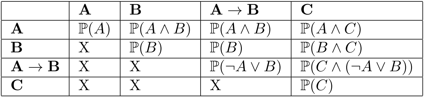
So we have the pairwise probabilities there. Note that there are two pairs of cells that are equivalent, so they ought to have the same probability, and that’s a first sanity check our algorithm must pass. Now let’s suppose we start with a prior probability of 0.5 to each of the above.

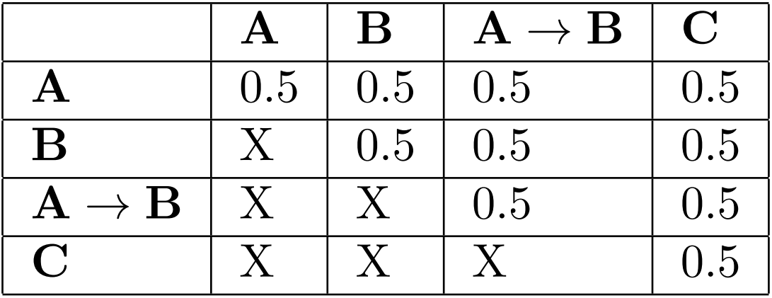
Clearly, this is incoherent, as you can check yourself by trying to apply the basic laws of probability to these numbers. So we want to turn that table into a coherent one. We use the following basic algorithm:

Identify the basic propositions ( $A$ , $B$ , $C$ , …) and their trivial equivalences.
Initialise a coherent joint distribution over them. Call this distribution $\mathbb Q$ .
Initialise update factors $\delta$ and $\varepsilon$ .
Initialise stopping factor $\mu$ .
Select a random element of the pairwise table, called here $\mathbb P(\phi)$ .
Set $\Delta \leftarrow \mathbb Q(\phi) - \mathbb P(\phi)$ .
If $\Delta = 0$ , go back to step 5. Otherwise, continue.
Set $\mathbb Q(\phi) \leftarrow min(max(\mathbb Q(\phi) - \varepsilon \Delta, 0), 1)$ .
If in the previous step $\mathbb Q(\phi)$ was set to $0$ or $1$ , set $\Delta \leftarrow \frac{\mathbb Q_{old}(\phi) - \mathbb Q_{new}(\phi)}{\varepsilon}$ .
Set $\mathbb P(\phi) \leftarrow \mathbb P(\phi) + \delta \Delta$ .
Update the rest of the $\mathbb Q$ table to maintain coherence.
If $\text{KL}(\mathbb P || \mathbb Q) > \mu$ (where the KL divergence is only taken where it’s defined) go back to step 5. Otherwise, output $\mathbb Q$ .

The idea behind this algorithm is to start with our known-to-be locally incoherent distribution and a known-to-be locally coherent distribution, then modify each in the direction of the other.

Actually, that’s not quite true. Since we guarantee $\mathbb Q$ remains coherent, we will have $\mathbb Q$ approaching $\mathbb P$ from within the space of coherent distributions, so not necessarily in the exact direction of $\mathbb P$ (who is not likewise constrained since it’s not coherent to start with).

When they’re “close enough” (using KL-divergence as our distance measure), we stop the algorithm, and we will have arrived at a $\mathbb P$ distribution that is in fact coherent. Ideally one would set $\delta \ll \varepsilon$ so that most of the modifications happen in $\mathbb Q$ distribution and the final distribution is as close to $\mathbb P$ as possible.

Step 11 is ill-defined, though. How do you “update the rest of the table to maintain coherence”?

Well, since $\mathbb Q$ is a full joint distribution, its entries must sum to $1$ . Therefore, we just effect the necessary changes in the affected rows. For example, if when running this algorithm it randomly picks the element $\neg A\lor B$ , then the elements of the table $\mathbb Q$ which will be affected are by that change are $\mathbb Q(\neg A\land B\land C)$ , $\mathbb Q(\neg A\land B\land \neg C)$ , $\mathbb Q(\neg A\land \neg B\land C)$ , $\mathbb Q(\neg A\land \neg B\land \neg C)$ , $\mathbb Q(A\land B\land C)$ , and $\mathbb Q(A\land B\land \neg C)$ ; a total of 6 entries out of the 8. So we subtract $\frac{\varepsilon\Delta}{6}$ from each of these entries, and we add $\frac{\varepsilon\Delta}{2}$ to each of the remaining two.

We initially ran this algorithm with $\delta = 0.01$ and $\varepsilon = 0.1$ and with an initial $\mathbb P(\phi) = 0.5$ for all $\phi$ . Then we tried the same priors but $\delta = 0.01$ and $\varepsilon = 0.1$ . I don’t have the actual values here and I’m too lazy to generate them, but the final tables were in fact coherent, close enough to the starting ones, and different amongst each other, which shows that choice of update parameters affects the results. We also tried a few different sets of sentences, with equally positive results. Different priors, naturally, give different results. And repeating the algorithm multiple times with the same input gives the same output, so yeah, cool.

There is an obvious problem, though. If I take, for instance, the above table, and use it as input to the algorithm again, a different table is generated. It is also coherent, but not the same one; so, let’s take the idea of $\delta \ll \varepsilon$ to its extreme. What if we set $\delta \leftarrow 0$ ?

Well, then we’re no longer guaranteed to terminate, with that termination condition on step 12. Our initial incoherent distribution $\mathbb P$ remains unchanged, and it’s only $\mathbb Q$ that moves, and they may never get close enough. However, we can modify step 12 to have the algorithm terminate if the two distributions are close enough or if at some step of the loop the KL divergence between the two raises instead of lowering.

Running this algorithm with different $\delta$ , as long as they’re sufficiently small, gives the same outputs. Using a previous output as a new input outputs the same table. So this version is more stable.

And a form of “logical updating” would be possible, whenever you found out logical relationships between the basic propositions. For instance, suppose we find out for a fact that $B \rightarrow \neg C$ . Then we can just add that as a column to our output $\mathbb Q$ with probability $1$ , and use that as the input.

This was about as far as we got to during the workshop.

Now what’s the obvious flaw in that algorithm?

What’s the size of the joint distribution? As I said above, with $n$ propositions, the table has $2^n$ entries. This algorithm then isn’t in P. It’s in the computable-but-intractable category, which is interesting, sure, and useful theoretically, but not quite something we could use.

And this is not a problem exclusive to Logical Uncertainty. Bayesian inference (like I explained above) is in general intractable; even approximate inference in a Bayesian network is.

However, what if $\mathbb Q$ was also a pairwise distribution, instead of the full joint? Then, we no longer would have an exponential number of steps when generating and when updating it, reducing it to a quadratic number of steps.

The problems, though, are how to generate a locally coherent $\mathbb Q$ and how to compute step 11. How do you calculate how much a change in $\mathbb Q(\neg A\lor B)$ affects $\mathbb Q(A)$ , or any other arbitrary pair of entries, without calculating the actual joint distribution?

I don’t know. My intuition says calculating this might be exponential, too, but I’m not sure. My intuition also says, however, that if we precompute how much changes in each entry of the pairwise $\mathbb Q$ affects the other entries, this would probably be less computationally expensive than the above method.

This is an interesting first step. A list of potential improvements to the algorithm would be:

Do not double-count trivially equivalent entries of the incoherent table. In other words, if two entries of the table are trivially equivalent, in step 5 of the algorithm we should not have a higher chance of selecting a sentence because it appears there multiple times.
Instead of reinitialising $\mathbb Q$ in step 2 of the algorithm whenever it’s run, we could use its previously calculated value/the algorithm’s previous output (or an extension thereof).
On step 11, we might use some other way to subtract/add different values to each entry of the $\mathbb Q$ matrix than just dividing them equally amongst the entries.

S	M	T	W	T	F	S
		1	2	3	4	5
6	7	8	9	10	11	12
13	14	15	16	17	18	19
20	21	22	23	24	25	26
27	28	29	30

What’s logical coherence for anyway?

Leave a comment Cancel reply

Recent Posts

Archives

Subscribe to Blog via Email

What’s logical coherence for anyway?

Share this:

Related

Leave a comment Cancel reply

Recent Posts

Archives

Subscribe to Blog via Email