I made a deck of Anki cards for this post - I think it is probably quite helpful for anyone who wants to deeply understand QACI. (Someone even told me they found the Anki cards easier to understand than the post itself)
You can have a look at the cards here, and if you want to study them, you can download the deck here.
Here are a few example cards:
Probabilities per element treat probability as an intensive property. I suggest: A distribution is a data structure carrying an expectation for every thing that depends on an x∈X.
So if X is [0;6], and the thing-depending-on-x is x², then the distribution concentrated on 5 has a 25 written there, the six-sided-die distribution has written there, and the uniform distribution has written there.
Halving an orange keeps its temperature/color/velocity, but halves what mass/energy/charge hang out there. An element has a property, but a quantity has an element.
Probability mass hangs out in timelines. should be "Take this x!", not "Are you x?", agree? Else this won't write itself and needs countability.
Is constrained mass M of similarpasts taken over a dot-product of functions that might have similar past w/each other?
something like that yes; something like a dot-product but of distributions over world-states, and those distributions are downstream of world-physics functions.
note that i'm not sure if i get what your comment is asking, let me know if i'm failing to answer your question.
this work was done by Tamsin Leake and Julia Persson at Orthogonal.
thanks to mesaoptimizer for his help putting together this post.
what does the QACI plan for formal-goal alignment actually look like when formalized as math? in this post, we'll be presenting our current formalization, which we believe has most critical details filled in.
1. math constructs
in this first part, we'll be defining a collection of mathematical constructs which we'll be using in the rest of the post.
1.1. basic set theory
we'll be assuming basic set theory notation; in particular, A×B×C is the set of tuples whose elements are respectively members of the sets A, B, and C, and for n∈N, Sn is the set of tuples of n elements, all members of S.
B={⊤,⊥} is the set of booleans and N is the set of natural numbers including 0.
given a set X, P(X) will be the set of subsets of X.
#S is the cardinality (number of different elements) in set S.
for some set X and some complete ordering <∈X2→B, min< and max< are two functions of type P(X)∖{∅}→X finding the respective minimum and maximum element of non-empty sets when they exist, using < as an ordering.
1.2. functions and programs
if n∈N, then we'll denote f∘n as repeated composition of f: f∘…∘f (n times), with ∘ being the composition operator: (f∘g)(x)=f(g(x)).
λx:X.B is an anonymous function defined over set X, whose parameter x is bound to its argument in its body B when it is called.
A→B is the set of functions from A to B, with → being right-associative (A→B→C is A→(B→C)). if f∈A→B→C, then f(x)(y) is simply f applied once to x∈A, and then the resulting function of type B→C being applied to y∈B. A→B is sometimes denoted BA in set theory.
AH→B is the set of always-halting, always-succeeding, deterministic programs taking as input an A and returning a B.
given f∈AH→B and x∈A, R(f,x)∈N∖{0} is the runtime duration of executing f with input x, measured in compute steps doing a constant amount of work each — such as turing machine updates.
1.3. sum notation
i'll be using a syntax for sums ∑ in which the sum iterates over all possibles values for the variables listed above it, given that the constraints below it hold.
x,y∑y=1y=xmod2x∈{1,2,3,4}x≤2
says "for any value of x and y where these three constraints hold, sum y".
1.4. distributions
for any countable set X, the set of distributions over X is defined as:
ΔX≔{f|f∈X→[0;1],x∑x∈Xf(x)≤1}
a function f∈X→[0;1] is a distribution ΔX over X if and only if its sum over all of X is never greater than 1. we call "mass" the scalar in [0;1] which a distribution assigns to any value. note that in our definition of distribution, we do not require that the distribution over all elements in the domain sums up to 1, but merely that it sums up to at most 1. this means that different distributions can have different "total mass".
we define Δ0X∈ΔX as the empty distribution: Δ0X(x)=0.
we define Δ1X∈X→ΔX as the distribution entirely concentrated on one element: Δ1X(x)(y)={1ify=x0ify≠x
we define NormalizeX∈ΔX→ΔX which modifies a distribution to make it sum to 1 over all of its elements, except for empty distributions:
NormalizeX(δ)(x)≔⎧⎪ ⎪ ⎪⎨⎪ ⎪ ⎪⎩δ(x)y∑y∈Xδ(y)ifδ≠Δ0X0ifδ=Δ0X
we define UniformX as a distribution attributing equal value to every different element in a finite set X, or the empty distribution if X is infinite.
UniformX(x)≔{1#Xif#X∈N0if#X∉N
we define maxΔX∈ΔX→P(X) as the function finding the elements of a distribution with the highest value:
maxΔX(δ)≔{x|x∈X,∀x′∈X:δ(x′)≤δ(x)}
1.5. constrained mass
given distributions, we will define a notation which i'll call "constrained mass".
it is defined as a syntactic structure that turns into a sum:
v1,…,vpv1,…,vpM[V]≔∑X1(x1)⋅…⋅Xn(xn)⋅Vx1:X1x1∈domain(X1)⋮⋮xn:Xnxn∈domain(Xn)C1C1⋮⋮CmCm
in which variables x are sampled from their respective distributions X, such that each instance of V is multiplied by X(x) for each x. constraints C and iterated variables v are kept as-is.
it is intended to weigh its expression body V by various sets of assignments of values to the variables v, weighed by how much mass the X distributions return and filtered for when the C constraints hold.
to take a fairly abstract but fully calculable example,
x,fM[f(x,2)]≔x,f∑(λn:{1,2,3}.n10)(x)⋅Uniform{min,max}(f)⋅f(x,2)x:λn:{1,2,3}.n10x∈domain(λn:{1,2,3}.n10)f:Uniform{min,max}f∈domain(Uniform{min,max})xmod2≠0xmod2≠0=x,f∑x10⋅12⋅f(x,2)x∈{1,2,3}f∈{min,max}xmod2≠0=1⋅min(1,2)10⋅2+3⋅min(3,2)10⋅2+1⋅max(1,2)10⋅2+3⋅max(3,2)10⋅2=1⋅1+3⋅2+1⋅2+3⋅320=1+6+2+920=1820=910
in this syntax, the variables being sampled from distributions are allowed to be bound by an arbitrary amount of logical constraints or new variable bindings below it, other than the variables being sampled from distributions.
1.6. bitstrings
B∗ is the set of finite bitstrings.
bitstrings can be compared using the lexicographic order <B∗, and concatenated using the ∥ operator. for a bitstring x∈B∗, |x|∈N is its length in number of bits.
for any countable set X, EncodeX∈X→B∗ and will be some reasonable function to convert values to bitstrings, such that ∀(x,y)∈X2:EncodeX(x)=EncodeX(y)⇔x=y. "reasonable" entails constraints such as:
1.7. cryptography
we posit σ≔B¯σ, the set of "signatures", sufficiently large bitstrings for cryptographic and uniqueness purposes, with their length defined as ¯σ=231 for now. this feels to me like it should be enough, and if it isn't then something is fundamentally wrong with the whole scheme, such that no manageable larger size would do either.
we posit a function ExpensiveHash∈B∗H→σ, to generate fixed-sized strings from seed bitstrings, which must satisfy the following:
at some point, we might come up with more formal ways to define ExpensiveHash in a way that checks that it isn't being computed inside Loc's f,g functions, nor inside the AI.
1.8. text and math evaluation
for any countable set X, we'll be assuming EvalMathX∈B∗→{{x}|x∈X}∪{∅} to interpret a piece of text as a piece of math in some formal language, evaluating to either:
for example,
EvalMathN("1+2")={3}EvalMathN("hello")=∅
1.9. kolmogorov simplicity
for any countable sets X and P:
K−X∈ΔX is some "kolmogorov simplicity" distribution over set X which has the properties of never assigning 0, and summing/converging to 1 over all of X. it must satisfy ∀x∈X:K−X(x)>0 and x∑x∈XK−X(x)=1.
K− is expected to give more mass to simpler elements, in an information-theoretic sense.
notably, it is expected to "deduplicate" information that appears in multiple parts of a same mathematical object, such that even if x∈B∗ holds lots of information, K−B∗(x) is not much higher (higher simplicity, i.e. lower complexity) to K−B∗×B∗(x,x).
we could define K−X similarly to cross-entropy, with some universal turing machine UTM∈B∗×N→B∗ returning the state of its tape after a certain number of compute steps:
i,nK−X≔NormalizeX(λx:X.∑1(2|i|⋅(n+1))2)i∈B∗n∈NUTM(i,n)=EncodeX(x)
kolmogorov simplicity over X with a prior from P, of type K−∼P,X:P→ΔX, allows elements it samples over to share information with a prior piece of information in P. it is defined as K−∼P,X(p)≔NormalizeX(λx:X.K−P×X(p,x)).
2. physics
in this section we posit some formalisms for modeling world-states, and sketch out an implementation for them.
2.1. general physics
we will posit some countable set Ω of world-states, and a distribution Ωα∈ΔΩ of possible initial world-states.
we'll also posit a function Ω→α∈Ω→ΔΩ which produces a distribution of future world-states for any specific world-state in the universe starting at α.
given an initial world-state α∈Ω, we'll call Ω→α(α) the "universe" that it gives rise to. it must be the case that ω∑ω∈ΩΩ→α(α)(ω)=1.
when α describes the start of a quantum universe, individual world-states Ω following it by Ω→α would be expected to correspond to many-worlds everett branches.
for concreteness's sake, we could posit Ω⊂B∗, though note that α is expected to not just hold information about the initial state of the universe, but also about how it is computed forwards.
given a particular α∈Ω:
finally, we define SimilarPastsα∈Ω×Ω→[0;1] which checks how much they have past world-states ωpast in common:
ω1SimilarPastsα(ω2,ω′2)≔M[Ω→α(ω1)(ω2)⋅Ω→α(ω1)(ω′2)]ω1:Ω→α(α)
2.2. quantum turing machines
we will sketch out here a proposal for Ω, Ωα, and Ω→ such that our world-state w has hopefully non-exponentially-small Ω→α(α)(ω).
the basis for this will be a universal quantum turing machine. we will posit:
we'll also define Δ2N∈ΔN as the "quadratic realityfluid distribution" which assigns diminishing quantities to natural numbers, but only quadratically diminishing: Δ2N(n)≔NormalizeN(1(n+1)2)
we can then define Ω→ as repeated applications of Step, with quadratically diminishing realityfluid:
n1,n2,sΩ→α(ω1)(ω2)≔c⋅M[s(n1,ω1)⋅s(n1+n2,ω2)]n1:Δ2Nn2:Δ2Ns(n,ω)=∥Step∘n(Δ1Ω(α))(ω)∥2
where the constant c is whatever scalar it needs to be for ω∑ω∈ΩΩ→α(α)(ω)=1 to be satisfied.
this implementation of Ω→α measures how much ω2 is in the future of ω1 by finding paths from α to ω1, and then longer paths from α to ω2.
and finally, we define Ωα as a distribution giving non-zero value to world-states (t,state0,0) where t is a tape where no negative-index cells are set to 1.
Ωα(t,s,i)≔⎧⎪ ⎪⎨⎪ ⎪⎩Δ2N(n∑n∈t2n)ifs=state0,i=0,t⊂N0otherwise
because we selected a universal (quantum) turing machine, there is at least one input tape implementing any single quantum algorithm, including the quantum algorithm implementing our physics.
3. implementing QACI
finally, we get into the core mechanisms of QACI.
the core idea of QACI is "blob location": mathematically formalizing the idea of locating our world and locating bitstrings (which i'll call "blobs") stored on computers within that world, out of the space of all possible computational universes, by sampling over functions which extract those blobs from world-states in Ω and functions which can produce a counterfactual world where that blob has been replaced with another blob of the same length (in number of bits).
3.1. question blob and observation
throughout these functions, we will posit the following constants:
μ1,μ2 are variables which will be passed around, called "observations". in normal AI agent framings, an AI would have a history of actions and observations, and decide on its next action based on that; but, in the one-shot framing we use, there is only a single action and a fixed set of observations. the observations, in practice, will be a very large pieces of data helping the AI locate itself in the multiverse of all possible computations, as well as get a better idea of how and where it is being ran. we will likely include in it things like:
μ1 will be produced before the question blob is generated, and μ2 will be produced after the question blob is generated but before the AI is launched.
3.2. overview
the overall shape of what we're doing can be seen on the illustration below: we start at the start of the universe α, and use four blob locations and a counterfactual blob function call to locate five other world-states. the illustration shows distributions of future and past world-states, as well as a particular sampling of for all four blob locations.
the location path from ωq′ to ωr is used to run QACI intervals, where counterfactual questions q′ are inserted and answers r are located in their future.
(we could also build fancier schemes where we locate the AI's returned action, or its code running over time, in order to "tie more tightly" the blob locations to the AI — but it is not clear that this helps much with blob location failure modes i'm concerned about.)
for the moment, we merely rely on μ1 and μ2 being uniquely identifying enough — though implementing them as static bitstrings might suffice, perhaps they could instead be implemented as lazily evaluated associative maps. when the AI tries to access members of those maps, code which computes or fetches information from the world (such as from the internet) would be executed determines the contents of that part of the observation object. this way, the observation would be conceptualized as a static object to the AI — and indeed it wouldn't be able to observe any mutations — but it'd be able to observe arbitrary amounts of the world, not just amounts we'd have previously downloaded.
we could make the QACI return not a scoring over actions but a proper utility function, but this only constrains the AI's action space and doesn't look like it helps in any way, including making QACI easier for the AI to make good guesses about. perhaps with utility functions we find a way to make the AI go "ah, well i'm not able to steer much future in world-states where i'm in hijacked sims", but it's not clear how or even that this helps much. so for now, the math focuses on this simple case of returning an action-scoring function.
3.3. blob location
for any blob length (in bits) n∈N:
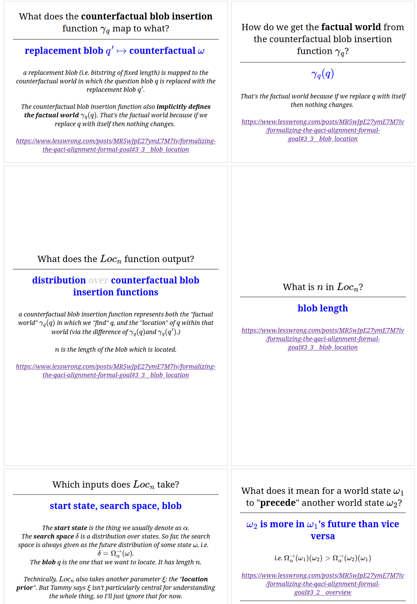
first, we'll posit Γn≔Bn→Ω the set of blob locations; they're identified by a counterfactual blob location function, which takes any counterfactual blob and return the world-state in which a factual blob has been replaced with that counterfactual blob.
Locn∈Ω×ΔΩ×Bn×Ξ→ΔΓn tries to locate an individual blob b (as a bitstring of length n) in a particular world-state sampled from the time-distribution (past or future) δ (which will usually be a distribution returned by Ω→α) within the universe starting at α.
it returns a distribution over counterfactual insertion functions of type Bn→Ω which take a counterfactual blob and return the matching counterfactual world-state. the elements in that distribution typically sum up to much less than 1; the total amount they sum up to corresponds to how much Loc finds the given blob in the given world-state to begin with; thus, sampling from a distribution returned by Loc in a constrained mass calculation M is useful even if said result is not used, because of its multiplying factor.
note that the returned counterfactual insertion function can be used to locate the factual world-state — simply give it the factual blob as input.
Ξ is some countably infinite set of arbitrary pieces of information which each call to Loc can use internally — the goal of this is for multiple different calls to Loc to be able to share some prior information, while only being penalized by K− for it once. for example, an element of Ξ might describe how to extract the contents of a specific laptop's memory from physics, and individual Loc calls only need to specify the date and the memory range. for concreteness, we can posit Ξ≔B∗, the set of finite bitstrings.
f,g,ω,b′,τLocn(α,δ,b,ξ)(γ)≔M[SimilarPastsα(ω,g(b′,τ))R(g,(b′,τ))+R(f,g(b′,τ))](f,g):K−∼Ξ,(ΩH→Bn×B∗)×(Bn×B∗H→Ω)(ξ)ω:λω:maxΔX(λω:Ω.{δ(ω)iff(ω)=(b,τ)0otherwise).δ(ω)b′:UniformBn∀b′′∈Bn:γ(b′′)=g(b′′,τ)f(γ(b′′))=(b′′,τ)
Loc works by sampling a pair of functions f,g, which convert world-states forth and back into {pairs whose first element is the blob and whose second element represents everything in the world-state except the blob}.
that latter piece of information is called τ (tau), and rather than being sampled τ is defined by the return value of f on the original world-state — notably, τ is not penalized for being arbitrarily large, though f and g are penalized for their compute time.
for a given fixed pair of f and g, Loc finds the set of hypothesis world-states ω with the highest value within the time-distribution δ for which f,g work as intended. this is intended to select the "closest in time" world-states in δ, to avoid adversarial attackers generating their own factual blobs and capturing our location.
it then weighs locations using, for every counterfactual blob b′∈Bn:
note that Locn, by design, only supports counterfactual blobs whose length n is equal to the length of the initial factual blob b — it wouldn't really make sense to talk about "replacing bits" if the bits are different.
in effect, Loc takes random f,g decoding and re-encoding programs, measures how complex and expensive they are and how far from our desired distributions are world-states in which they work, and how close to the factual world-state their counterfactual world-states are.
3.4. blob signing
we'll define Π≔B|q|−¯σ, the set of possible answer bitstring payloads.
counterfactual questions will not be signed, and thus will be the set of bitstrings of the same length as the factual question — B|q|.
we'll define Sign∈Π×B∗→B|q| as Sign(π,k)≔ExpensiveHash(π∥k)∥π. this functions tags blob payloads using a "signature" generated from a seed bitstring, concatenating it to the blob payload.
3.5. action-scoring functions
we will posit A⊂B∗ as the finite set of actions the AI can take, as a finite set of bitstrings.
we'll call U≔A→[0;1] the set of "scoring functions" over actions — functions which "have an opinion" about various actions. this is similar to utility functions, except it's over actions rather than over worlds or world-histories.
they can be composed using Compose∈ΔU→U, which could be simple scoring-function averaging:
uCompose(δ)(a)?≔M[u(a)]u:δ
but alternatively, we could use something like Diffractor's Rose bargaining to reduce the ability for scoring/utility functions to threaten each other — and notably ours.
Compose?≔Rose
(where i'm using ?≔ to mean "maybe define this way, but i'm not sure")
3.6. QACI query
using those, we define QACI∈Ω×Γ|q|×Ξ×B|q|→ΔΠ which given a physics hypothesis α, a question blob location γq, and a blob location prior ξ, returns the highest guess returned answer payload πr for a given counterfactual question q′.
γrQACI(α,γq,ξ,q′)(πr)≔M[1]γr:Loc|q|(α,Ω→α(γq(q′)),Sign(πr,q′),ξ)
QACI works by sampling answer blob locations γr, from world-states in the future of the counterfactual question world-state γq(q′), signed using q′.
with its first three parameters fixed, QACI becomes the straightforward counterfactual query function B|q|→ΔΠ: one can call it with arbitrary counterfactual text inputs (within the size limitation), and get a distribution over possible answers, which can easily be collapsed using maxΔΠ.
3.7. top-level QACI call
the top-level call to the QACI query function, QACI0∈Ω×Γ|q|×Ξ→ΔU interprets its output as a piece of math and executes it with, as parameters, various global and contextual values it might need access to, and returns a distribution over action-scoring functions:
πr,fQACI0(α,γq,ξ)(u)≔M[1]πr:QACI(α,γq,ξ,q′0)f∈EvalMath{q}×{μ1}×{μ2}×Ω×Γ|q|×Ξ→U(πr)f(q,μ1,μ2,α,γq,ξ)=u
where q′0∈B|q| is the initial counterfactual blob, such as "return a good scoring of actions" encoded in ASCII, padded with zeros to be of the right length.
QACI0's distribution over answers demands that the answer payload πr, when interpreted as math and with all required contextual variables passed as input (q,μ1,μ2,α,γq,ξ), returns an action-scoring function equal to u — this is how it measures the weight of any action-scoring function u.
M[1] makes it that QACI0's distributions are only determined by the sampled variables and logical requirements.
EvalMath's f function having access to QACI's distribution over output texts rather than best candidate allows it to discard as many invalid candidates as it needs and stick to ones that match whatever constraits it has.
3.8. action scoring
we'll posit the AI as AI∈U→A — a program which tries to satisfy a scoring over actions, by making a high-expected-score guess.
we define Score∈U, the action-scoring function which the AI will be making guesses about as a scoring function over actions, which happens to be one that is, hopefully, good. this is the scoring function for which the AI will be trying to produce an action that is as favorable as possible, within its limited capabilities.
α,ξ,γμ1,γμ2,γqScore≔Compose(λu:U.M[NormalizeU(QACI0(α,γq,ξ))(u)])α:Ωαξ:K−Ξγμ1:Loc|μ1|(α,Ω→α(α),μ1,ξ)γμ2:Loc|μ2|(α,Ω→α(γμ1(μ1)),μ2,ξ)γq:Loc|q|(α,Ω→α(γμ1(μ1)),q,ξ)Ω→α(γq(q))(γμ2(μ2))>Ω→α(γμ2(μ2))(γq(q))
where the following variables are sampled:
and the world-state containing the second observation μ2 is required to be in the future of the word-state containing the question q.
then, we rate possible actions a by composing the scoring functions produced by QACI0 for all of those blob location hypotheses.
for any question location, the set of action-scoring functions sampled by QACI0 is normalized. this is because pairs of AI-action location and question location should not be penalized for having a "harder to find" answer — once the observations and question have been located, we want to obtain the answer no matter what.
finally, we'll just execute the action returned by AI(Score).