ProLU: A Nonlinearity for Sparse Autoencoders

Glen Taggart

Crossposted from the AI Alignment Forum. May contain more technical jargon than usual.

Abstract

This paper presents , an alternative to $ReLU$ for the activation function in sparse autoencoders that produces a pareto improvement over both standard sparse autoencoders trained with an L1 penalty and sparse autoencoders trained with a Sqrt(L1) penalty.

ProLU (m_{i}, b_{i}) = {\begin{matrix} m_{i} & if m_{i} + b_{i} > 0 and m_{i} > 0 0 & otherwise \end{matrix}

{SAE}_{ProLU} (x) = ProLU ((x - b_{d e c}) W_{e n c}, b_{e n c}) W_{d e c} + b_{d e c}

The gradient wrt. $b$ is zero, so we generate two candidate classes of differentiable $ProLU$ :

${ProLU}_{R e L U}$
- $\frac{\partial^{*} {ProLU}_{R e L U} (m_{i}, b_{i})}{\partial b_{i}} = \frac{\partial {ProLU}_{R e L U} (m_{i}, b_{i})}{\partial m_{i}} = {\begin{matrix} 1 & if m_{i} + b_{i} > 0 and m_{i} > 0 0 & otherwise \end{matrix}$
${ProLU}_{S T E}$
- $\frac{\partial^{*} {ProLU}_{S T E} (m_{i}, b_{i})}{\partial m_{i}} = {\begin{matrix} 1 + m_{i} & if m_{i} > 0 and m_{i} + b_{i} > 0 0 & otherwise \end{matrix}$
- $\frac{\partial^{*} {ProLU}_{S T E} (m_{i}, b_{i})}{\partial b_{i}} = {\begin{matrix} m_{i} & if m_{i} > 0 and m_{i} + b_{i} > 0 0 & otherwise \end{matrix}$

PyTorch Implementation

Introduction

SAE Context and Terminology

Learnable parameters of a sparse autoencoder:

$W_{e n c}$ : encoder weights
$W_{d e c}$ : decoder weights
$b_{e n c}$ : encoder bias
$b_{d e c}$ : decoder bias

The output of an SAE is given by

S A E (x) = ReLU ((x - b_{d e c}) W_{e n c} + b_{e n c}) W_{d e c} + b_{d e c}

Training

Notation: Encoder/Decoder
Let
$encode (x) = ReLU ((x - b_{d e c}) W_{e n c} + b_{e n c})$ $decode (a) = a W_{d e c} + b_{d e c}$
so that the full computation done by an SAE can be expressed as
$SAE (x) = decode (encode (x))$

An SAE is trained with gradient descent on

L_{t r a i n} = | | x - S A E (x) | |_{2}^{2} + λ P (encode (x))

where $λ$ is the sparsity penalty coefficient (often "L1 coefficient") and $P$ is the sparsity penalty function, used to encourage sparsity.

$P$ is commonly the L1 norm $| | a | |_{1}$ but recently $P (a) = | | a | |_{\frac{1}{2}}^{\frac{1}{2}}$ has been shown to produce a Pareto improvement on the L0 and CE metrics. We will use this as a further baseline to compare against when assessing our models in addition to the standard $ReLU$ -based SAE with L1 penalty.

Motivation: Inconsistent Scaling in Sparse Autoencoders

Due to the affine translation, sparse autoencoder features with nonzero encoder biases only perfectly reconstruct feature magnitudes at a single point.

This poses difficulties if activation magnitudes for a fixed feature tend to vary over a wide range. This potential problem motivates the concept of scale consistency:

A scale consistent response curve

The bias maintains its role in noise suppression, but no longer translates activation magnitudes when the feature is active.

The lack of gradients for the encoder bias term poses a challenge for learning with gradient descent. This paper will formalize an activation function which gives SAEs this scale-consistent response curve, and motivate and propose two plausible synthetic gradients, and compare scale-consistent models trained with the two synthetic gradients to standard SAEs and SAEs trained with Sqrt(L1) penalty.

Scale Consistency Desiderata

Notation: Centered Submodule
The use of the decoder bias can be viewed as performing centering on the inputs to a centered SAE then reversing the centering on the outputs:
$S A E (x) = S A E_{c e n t} (x - b_{d e c}) + b_{d e c}$

$S A E_{c e n t} (x) = ReLU (x W_{e n c} + b_{e n c}) W_{d e c}$

Notation: Specified Feature
Let $W^{i}$ denote the weights and $b_{e n c}^{i}$ the encoder bias for the $i$ -th feature. Then, let
$S A E^{i} (x) = S A E_{c e n t}^{i} (x - b_{d e c}) + b_{d e c}$

$where S A E_{c e n t}^{i} (x) = ReLU (x W_{e n c}^{i} + b_{e n c}^{i}) W_{d e c}^{i}$

Conditional Linearity

1. S A E_{c e n t}^{i} (v_{1}) > 0 \land S A E_{c e n t}^{i} (v_{2}) > 0 ⟹ S A E_{c e n t}^{i} (v_{1}) + S A E_{c e n t}^{i} (v_{2}) = S A E_{c e n t}^{i} (v_{1} + v_{2})

2. \forall v S A E_{c e n t}^{i} (v) > 0 \land k > 1 ⟹ S A E_{c e n t}^{i} (k v) = k \cdot S A E_{c e n t}^{i} (v)

Noise Suppresion Threshold

3. b_{e n c} < 0 ⟹ \exists η \in (0, \infty) \forall ϵ \in (0, \infty) s.t. S A E_{c e n t}^{i} (η \cdot v) = 0 \land S A E_{c e n t}^{i} ((η + ϵ) \cdot v) > 0

Proportional ReLU $(ProLU)$

We define the Proportional ReLU $(ProLU)$ as:

ProLU (m_{i}, b_{i}) = {\begin{matrix} m_{i} & if m_{i} + b_{i} > 0 and m_{i} > 0 0 & otherwise \end{matrix}

Backprop with $ProLU$ :

To use $ProLU$ in SGD-optimized models, we first address the lack of gradients wrt. the $b$ term.

$ReLU$ gradients:

For comparison and later use, we will first consider $ReLU$ : partial derivatives are well defined for $ReLU$ at all points other than $x_{i} = 0$ :

\frac{\partial ReLU (x_{i})}{\partial x_{i}} = {\begin{matrix} 1 & if x_{i} > 0 0 & if x_{i} < 0 \end{matrix}

Gradients of $ProLU$ :

Partials of $ProLU$ wrt. $m$ are similarly well defined:

\frac{\partial ProLU (m_{i}, b_{i})}{\partial m_{i}} = {\begin{matrix} 1 & if m_{i} + b_{i} > 0 and m_{i} > 0 0 & otherwise \end{matrix}

However, they are not well defined wrt. $b$ , so we must synthesize these.

Methods

Notation: Synthetic Gradients
Let $\frac{\partial^{*} f}{\partial x}$ denote the synthetic partial derivative of $f$ wrt. $x$ , and $\nabla^{*} f$ the synthetic gradient of f, used for backpropagation as a stand-in for the gradient.

Different synthetic gradient types

We train two classes of $ProLU$ with different synthetic gradients. These are distinguished by their subscript:

${ProLU}_{R e L U}$
${ProLU}_{S T E}$

They are identical in output, but have different synthetic gradients. I.e.

{ProLU}_{R e L U} (m, b) = {ProLU}_{S T E} (m, b)

\nabla^{*} {ProLU}_{R e L U} (m, b) \equiv̸ \nabla^{*} {ProLU}_{S T E} (m, b)

Defining ${ProLU}_{R e L U}$ : $ReLU$ -like gradients

The first synthetic gradient is very similar to the gradient for $ReLU$ . We retain the gradient wrt. $m$ , and define the synthetic gradient wrt. $b$ to be the same as the gradient wrt. $m$ :

\frac{\partial^{*} {ProLU}_{R e L U} (m_{i}, b_{i})}{\partial b_{i}} = \frac{\partial {ProLU}_{R e L U} (m_{i}, b_{i})}{\partial m_{i}} = {\begin{matrix} 1 & if m_{i} + b_{i} > 0 and m_{i} > 0 0 & otherwise \end{matrix}

Defining ${ProLU}_{S T E}$ : Derivation from straight-through estimator

The second class of $ProLU$ uses synthetic gradients for both $b$ and $m$ and can be motivated by framing $ProLU$ and $ReLU$ in terms of the threshold function, and a common choice of straight-through estimator (STE) for the threshold function. This is a plausible explanation for the observed empirical performance but it should be noted that there are many degrees of freedom and possible alternative

Setup

The threshold function $Thresh$ is defined as follows:

Thresh (x) = {\begin{matrix} 1 & if x > 0 0 & otherwise \end{matrix}

We will rephrase the partial derivative of $ReLU$ in terms of the threshold function for ease of later notation:

\frac{\partial ReLU (x_{i})}{\partial x_{i}} = {\begin{matrix} 1 & if x_{i} > 0 0 & if x_{i} < 0 \end{matrix} = Thresh (x_{i})

It is common to use a straight-through estimator (STE) to approximate the gradient of the threshold function:

\frac{\partial^{*} Thresh (x_{i})}{\partial x_{i}} = S T_{Thresh} (x_{i})

We can reframe $ProLU$ in terms of the threshold function:

ProLU (m_{i}, b_{i}) = ReLU (m_{i}) \cdot Thresh (m_{i} + b_{i})

Synthetic Gradients wrt. $m$

Now, we take partial derivatives of $ProLU$ wrt. $m$ using the STE approximation for the threshold function:

\frac{\partial^{*} {ProLU}_{S T E} (m_{i}, b_{i})}{\partial m_{i}} = \frac{\partial^{*}}{\partial m_{i}} (ReLU (m_{i}) \cdot Thresh (m_{i} + b_{i}))

= \frac{\partial ReLU (m_{i})}{\partial m_{i}} \cdot Thresh (m_{i} + b_{i}) + ReLU (m_{i}) \cdot \frac{\partial^{*} Thresh (m_{i} + b_{i})}{\partial m_{i}}

= Thresh (m_{i}) \cdot Thresh (m_{i} + b_{i}) + ReLU (m_{i}) \cdot S T_{Thresh} (m_{i} + b_{i})

= Thresh (m_{i}) \cdot Thresh (m_{i} + b_{i}) + m_{i} Thresh (m_{i}) \cdot S T_{Thresh} (m_{i} + b_{i})

Synthetic Gradients wrt. $b$

\frac{\partial^{*} {ProLU}_{S T E} (m_{i}, b_{i})}{\partial b_{i}} = \frac{\partial^{*}}{\partial b_{i}} (ReLU (m_{i}) \cdot Thresh (m_{i} + b_{i}))

= \frac{\partial ReLU (m_{i})}{\partial b_{i}} \cdot Thresh (m_{i} + b_{i}) + ReLU (m_{i}) \cdot \frac{\partial^{*} Thresh (m_{i} + b_{i})}{\partial b_{i}}

= 0 \cdot Thresh (m_{i} + b_{i}) + ReLU (m_{i}) \cdot S T_{Thresh} (m_{i} + b_{i})

= m_{i} Thresh (m_{i}) \cdot S T_{Thresh} (m_{i} + b_{i})

Choice of Straight-Through Estimator

There are many possible functions to use for $S T_{Thresh} (x)$ . In our experiments, we take the derivative of $ReLU$ as the choice of straight-through estimator. This choice has been used in training quantized neural nets.

$S T_{Thresh} (x) := Thresh (x)$

then, synthetic gradients wrt. $m$ are given by,

\frac{\partial^{*} {ProLU}_{S T E} (m_{i}, b_{i})}{\partial m_{i}} = Thresh (m_{i}) \cdot Thresh (m_{i} + b_{i}) + m_{i} Thresh (m_{i}) \cdot Thresh (m_{i} + b_{i})

= (1 + m_{i}) \cdot Thresh (m_{i}) \cdot Thresh (m_{i} + b_{i})

= {\begin{matrix} 1 + m_{i} & if m_{i} > 0 and m_{i} + b_{i} > 0 0 & otherwise \end{matrix}

and wrt. $b$ are given by,

\frac{\partial^{*} {ProLU}_{S T E} (m_{i}, b_{i})}{\partial b_{i}} = m_{i} Thresh (m_{i}) \cdot Thresh (m_{i} + b_{i})

= {\begin{matrix} m_{i} & if m_{i} > 0 and m_{i} + b_{i} > 0 0 & otherwise \end{matrix}

$ProLU$ Sparse Autoencoder

We can express the encoder of a $ProLU$ SAE as

{encode}_{ProLU} (x) = ProLU ((x - b_{d e c}) W_{e n c}, b_{e n c})

No change is needed to the decoder. Thus,

{SAE}_{ProLU} (x) = decode ({encode}_{ProLU} (x))

Experiment Setup

Shared among all sweeps:

Adam optimizer, with:
- $β_{1} = 0.9, β_{2} = 0.999$
$batch size = 4096$
Data
- Trained on gpt2 layer 6 pre-residual activations
- Tokens: ~400m tokens from The Pile @ack(Alan Cooney's pre-tokenized pile)
- -> ~100k gradient steps
LR schedule
- Warmup for $\frac{2}{1 - β_{2}} = 2, 000$ steps in accordance with On the adequacy of untuned warmup for adaptive optimization
- Linear warmup after each resample. Same value 2,000
- Linear cooldown to 1/10 initial value over 20,000 steps starting at 75,000 steps
Anthropic resampling
- I used 3e-6 as the dead threshold rather than 0
- Resample at 25,000 and 50,000 steps
- The proportion of the average encoder norm resampled to varied between sweeps
Normalization:
- L2 normalization as proposed by Anthropic
SAE details
- Dictionary expansion factor of 16
- Tied decoder bias, untied encoder/decoder weights

Varying between sweeps:

Experiment 1:
- $l r = 0.001$
- 30 total runs
- Resampled to 0.02 of avg encoder norm
Experiment 2:
- $l r = 0.0003$
- 48 total runs
- Resampled to 0.02 of avg encoder norm
Experiment 3:
- $l r = 0.001$
- 30 total runs
- Resampled to 0.2 of avg encoder norm
- adjusted L1-coefficient ranges for each model, to get more overlap in L0 ranges.
  - different architectures respond very differently to l1 coefficients

Varying within sweeps

L1 coefficient
Architecture choice of nonlinearity:
- $ReLU$
- ${ProLU}_{R e L U}$
- ${ProLU}_{S T E}$
L1 Penalty type
- L1: $P (a) = | | a | |_{1}$
- Sqrt(L1): $P (a) = | | a | |_{1 / 2}^{1 / 2}$

Results

Let:
$L_{m o d e l}$ be the CE loss of the model unperturbed on the data distribution
$L_{r e c o n s t r u c t e d}$ be the CE loss of the model when activations are replaced with the reconstructed activations
$L_{z e r o}$ be the CE loss of the model when activations are replaced with the zero vector

Degradation: or Information Lost. This measures how much information about the correct next token the model loses by having its activations $a$ replaced with the SAE's reconstruction $SAE (a)$ .
$degradation = L_{r e c o n s t r u c t e d} - L_{m o d e l}$

For $L 0 < 25$ :

The pareto-best architecture uses the ${ProLU}_{S T E}$ nonlinearity with an L1 sparsity penalty.

For $L 0 > 25$ :

There are no occurrences of models using ${ProLU}_{S T E}$ with L1 penalty in this L0 range
Of the remaining models, ${ProLU}_{ReLU}$ with Sqrt(L1) penalty is pareto-best.

Further Investigation

MSE/L1 Pareto Frontier

The gradients of $ProLU$ are not the gradients of the loss landscape, so it would be a reasonable default to expect these models to perform worse than a vanilla SAE. Indeed I expect they may perform worse on the optimization target, and that the reason why this is able to work is there is slack in the problem introduced by us being unable to optimize for our actual target directly -- our current options are to optimize for L1 or Sqrt(L1) as sparsity proxies for what we actually want because L0 is not a differentiable metric.

Actual target: minimize L0 and bits lost
Optimization (proxy) target: minimize L1 (or $\sqrt{L 1}$ )) and MSE

Because we're not optimizing for the actual target, I am not so surprised that there may be weird tricks we can do to get more of what we want.

On this vein of thought, my prediction after seeing the good performance on the actual target (and prior to checking this prediction) was:

Despite improved performance on degradation/L0 ProLU SAEs will have the same or worse on the MSE/L1 curve.
We may also see the higher performing architectures have greater L1/L0

Let's check:
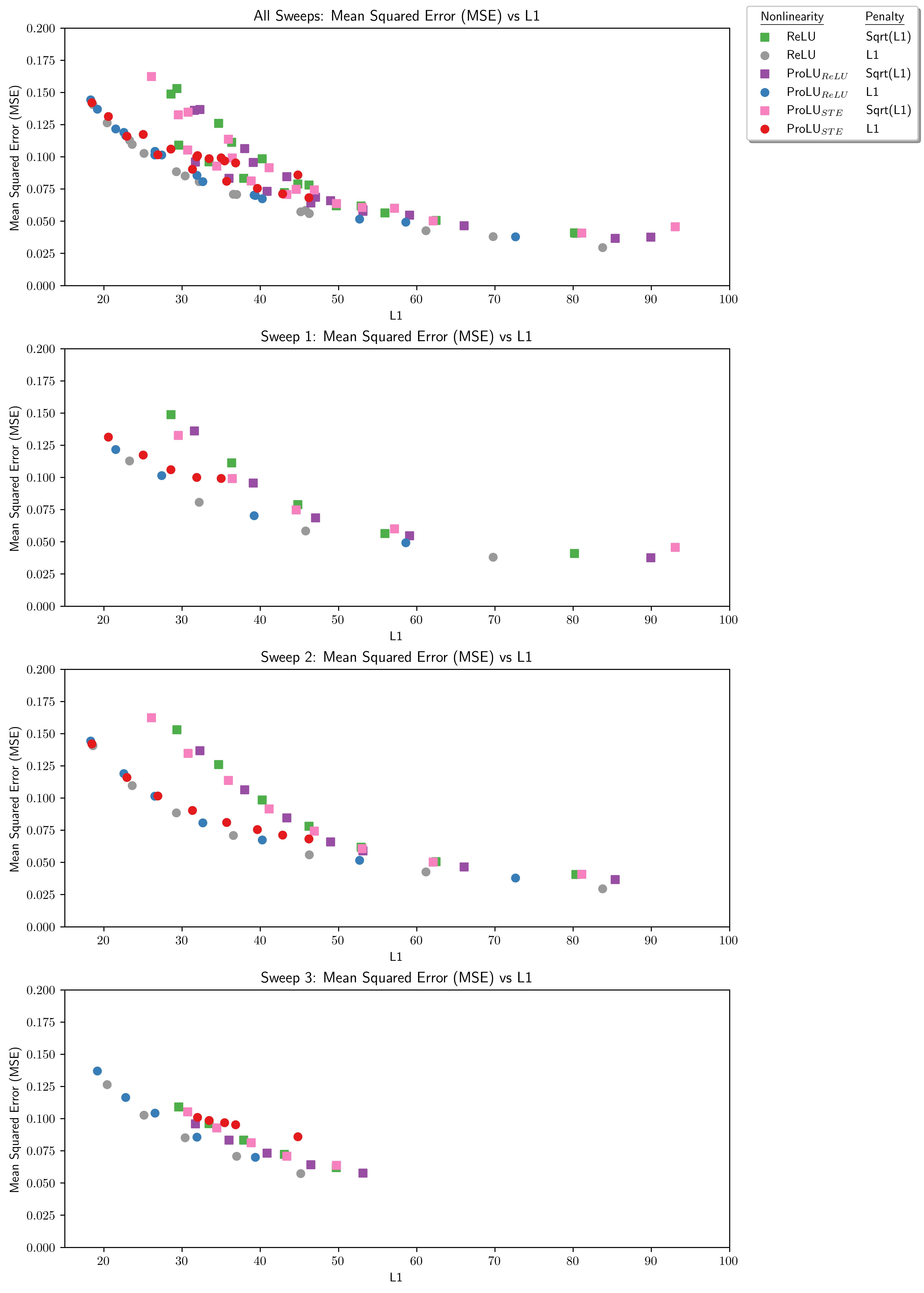In favor of the hypothesis, while other architectures sometimes join it on the frontier, the Vanilla ReLU is present for the entirety of this Pareto frontier. On the other hand, at lower sparsity levels ${ProLU}_{S T E}$ joins it at the frontier. So the part where this change does not improve performance on the optimization target seems true, but it's not clear that better performance on the actual target is coming from worse performance on the optimization target.

This suggests a possible reason for why the technique works well:
Possibly the gains from this technique do not come from scale consistency so much as that it forced us to synthesize some gradients and those gradients happened to point more in the direction of what we actually want.

Here is the graph of L1 norm versus L0 norm:

This looks like it's possible that what is working well here is the learned features are experiencing less suppression, but that may not be the only thing going on fixing this. Feature suppression is still consistent with the scale consistency hypothesis, as consistent undershooting would be an expected side effect if that is a real problem, since regular SAEs may be less able to filter unwanted activations if they are keeping biases near zero in order to minimize errors induced by scale inconsistency.

More investigation is needed here to create a complete or confident picture of what is cause of the performance gains in $ProLU$ SAEs.

Unfortunately, I did not log $\sqrt{L 1}$ so I can't compare with that curve, but could load the models to create those graphs in follow-up work.

Acknowledgements

Noa Nabeshima and Arunim Agarwal gave useful feedback and editing help on the draft of this post.

Mason Krug for in depth editing of my grant proposal, which helped seed this writeup and clarify my communication.

How to Cite

@misc{ProLUNonlinearity,
   title = {ProLU: A Nonlinearity for Sparse Autoencoders},
   author = {Glen M. Taggart},
   year = {2024},
   howpublished = {\url{https://www.alignmentforum.org/posts/HEpufTdakGTTKgoYF/prolu-a-nonlinearity-for-sparse-autoencoders}},
}

[-]wuthejeff9dΩ340

This is great! We were working on very similar things concurrently at OpenAI but ended up going a slightly different route.

A few questions:
- What does the distribution of learned biases look like?
- For the STE variant, did you find it better to use the STE approximation for the activation gradient, even though the approximation is only needed for the bias?

[-]Glen Taggart8dΩ110

Thank you!

That's super cool you've been doing something similar. I'm curious to see what direction you went in. It seemed like there's a large space of possible things to do along these lines. DeepMind also did a similar but different thing here.

What does the distribution of learned biases look like?

That's a great question, something I didn't note in here is that positive biases have no effect on the output of the SAE -- so, if the biases were to be mostly positive that would suggest this approach is missing something. I saved histograms of the biases during training, and they generally look to be mostly (80-99% of bias values I feel like?) negative. I expect the exact distributions vary a good bit depending on L1 coefficient though.

I'll post histograms here shortly. I also have the model weights so I can check in more detail or send you weights if you'd like either of those things.

On a related point, something I considered: since positive biases behave the same as zeros, why not use ProLU where the bias is negative and regular ReLU where the biases are positive? I tried this, and it seemed fine but it didn't seem to make a notable impact on performance. I expect there's some impact, but like a <5% change and I don't know in which direction, so I stuck with the simpler approach. Plus, anyways, most of the bias values tend to be negative.

For the STE variant, did you find it better to use the STE approximation for the activation gradient, even though the approximation is only needed for the bias?

I think you're asking whether it's better to use the STE gradient only on the bias term, since the mul () term already has a 'real gradient' defined. If I'm interpreting correctly, I'm pretty sure the answer is yes. I think I tried using the synthetic grads just for the bias term and found that performed significantly worse (I'm also pretty sure I tried the reverse just in case -- and that this did not work well either). I'm definitely confused on what exactly is going on with this. The derivation of these from the STE assumption is the closest thing I have to an explanation and then being like "and you want to derive both gradients from the same assumptions for some reason, so use the STE grads for $m$ too." But this still feels pretty unsatisfying to me, especially when there's so many degrees of freedom in deriving STE grads:

choice of STE
I glossed over this but it seems like maybe we should think of the grads of $Thresh$ like $\frac{\partial^{*} Thresh (x)}{\partial x} = k \cdot ST (x)$ where $k > 0$
- I think this because $Thresh (x)^{n} = Thresh (x)^{m}$ for $n, m > 1$
- I also see an argument from this that $Thresh (x)$ should be a term in the partial of $Thresh$ , which is a property I like about taking $Thresh (x)$ as it's own derivative

Another note on the STE grads: I first found these gradients worked emperically, was pretty confused by this, spent a bunch of time trying to find an intuitive explanation for them plus trying and failing to find a similar-but-more-sensible thing that works better. Then one night I realized that those exact gradient come pretty nicely from these STE assumptions, and it's the best hypothesis I have for "why this works" but I still feel like I'm missing part of the picture.

I'd be curious if there are situations where the STE-style grads work well in a regular ReLU, but I expect not. I think it's more that there is slack in the optimization problem induced by being unable to optimize directly for L0. I think it might be just that the STE grads with L1 regularization point more in the direction of L0 minimization. I have a little analysis I did supporting this I'll add to the post when I get some time.

LESSWRONG
LW