Thanks for making this, it's good to see high-effort critiques.
Let’s start with a plot that shouldn’t be too surprising. Four reasonable models fit the METR data equally well. They agree about the past but disagree strongly about the future.
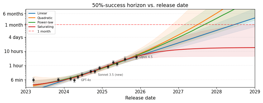
Note that we have data going back to 2019 (GPT-2), and it looks like the other models wouldn't fit the earlier trend well. (The raw data should be in the time horizons 1.0 folder). I'd guess the best fitting models over the whole range would be linear and a slightly superlinear power law.
METR also cares about 80% success and fits a separate model for that.
Actually it's worse than that; we just get the 80% point of the logistic. Initially 80% success was an afterthought, but since it's clear people care about it, Alex Barry has been doing Bayesian analysis that supports it.
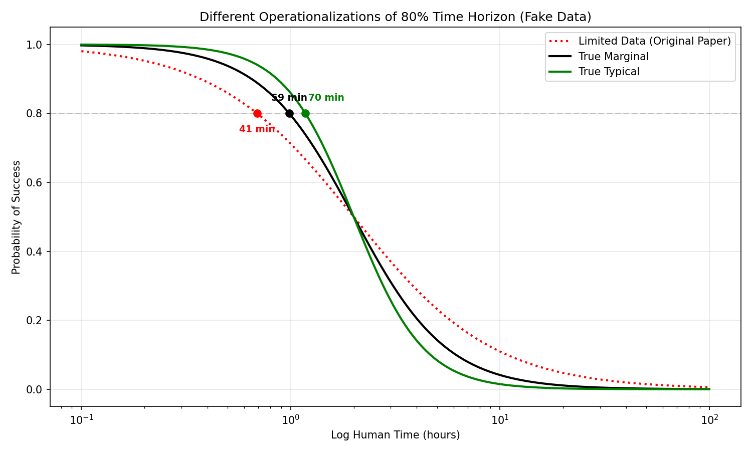
But there are actually two reasonable ways to define “80% success,” and they give different answers.
- Typical: Pick a task of average difficulty for its length. Can the model solve it 80% of the time? This is roughly what METR computes.
- Marginal: Pick a random task of that length. What’s the expected success rate? Because some tasks are much harder than average, the hard ones drag down the average more than easy ones push it up.
Our method is actually closer to computing "Marginal", because when fitting the logistic curve, the points near x = 1 hour include all trials for all tasks estimated at that length. We didn't actually have the means to get the "Typical" 80% point since we don't compute "average difficulty for its length" anywhere.
In your analysis, the "Typical" 80% time horizon of the last point (I think Claude 4.5 Opus) is around 110 minutes, whereas ours is 42 minutes. I'm not sure what makes the marginal so low in your analysis (5 minutes) but Alex suggests it might be that
Basically there are two factors that change the original analysis vs "typical"
- We have limited baseline data (often 0-2 baselines per task), so our time estimates will be noisy estimates of the average human time.
- Tasks that take humans the same average time will still differ in difficulty (this is "typical" vs "marginal").
If we were able to account for each of the factors or estimate them using stats, our data model would get more predictive, the slopes increase, and the 80% time horizon increase from our results -> "marginal" -> "typical". But like you say we actually want to stop at "marginal".
I chatted with Thomas a bit about this, and I also agree that the default METR model should also output things that are close to the 'marginal' definition of time horizon (or at least as well as it can be approximated with the inverse logit sigmoid).
I think the important thing to realise is that while one needs to take additional steps for the 'marginal' approach when fitting a model that explicitly accounts for the deviation in task-length-for-humans vs task-difficulty-for-llms, models that don't explicitly account for this (such as the original METR model) should have it naturally learned into the shape of their logistic curve.
(A similar thing is also true for having the discrimination parameter vary by task instead of by model - if it varies by task this uncertainty needs to be accounted for in the time horizon calculations, but since this is not the case in the original METR model it does not).
I think the important thing to realise is that while one needs to take additional steps for the 'marginal' approach when fitting a model that explicitly accounts for the deviation in task-length-for-humans vs task-difficulty-for-llms, models that don't explicitly account for this (such as the original METR model) should have it naturally learned into the shape of their logistic curve.
I don't immediately see this. The marginal idea is roughly about integrating over random effects, and that's hard to capture without actually doing it. My statement that METR's original approach is about the typical effect is wrong though.
I think we agree and I just stated this badly - I was just meaning to say that METR's original approach is closer to marginal despite them not explicitly doing the integrating over the random effects (although I agree you need to do integrate over the random effects in models that include them to get the marginal time horizon).
Note that we have data going back to 2019 (GPT-2), and it looks like the other models wouldn't fit the earlier trend well. (The raw data should be in the time horizons 1.0 folder). I'd guess the best fitting models over the whole range would be linear and a slightly superlinear power law.
Thanks, I didn't think of checking of this! I refitted the models to all the data in the updated post. The story doesn't really change much when it comes to fit. I also think it's ok, probably preferable, to use only v1.1. There's not much reason to go back this far, especially due to the well-known kink which happens roughly at the start of v1.1 anyway.
Actually it's worse than that; we just get the 80% point of the logistic.
Hmmm... Yeah, I gotta admit I didn't really check how you did this. I'm not sure what this means in practice and would careful interpreting it. It doesn't clearly map to either typical or marginal. Marginal seems intuitively out of the question because it requires integration over random effects though. It's just something else entirely, no?
Ideally, I think the curves would look something like this: [...]
I had Claude make some plots at the updated post that shows the corresponding curves in my model. I don't have a strong opinion of what the plots should ideally look like, as its kinda open how even perfectly estimated human times (
Anyway, the difference between marginal and typical in my plots are pretty well-explained from the residuals plot, as it has to take into account the scattering of the residuals (and we have a sizable proportion of tasks with equivalent time 22x as large!). Is this the close to the "true marginal"? I mean, yes, it is, IF we take human completion time in the data set as being true. If we don't, then we have to model it.
To estimate the marginal stuff properly we need to model the baseline times. I didn't really try this, and I do think a good implementation would use all the available data, not only the columns on the Github. But it is possible to slap a lognormal on the public data too, but one data point per task is not enough to gain a lot of information, and our results will be very prior-driven. And honestly I think that's where we are wrt to 80% horizons anyway.
Thanks for the great writeup!
I'm a statistician who does some work with METR, and I recently worked on a very similar project to create a Bayesian version of the Time Horizon model. Mine ended up being somewhat different to yours (mine deviates a bit more from the currently structure of the METR model), but its great to see other people stress testing modelling.
On the 80% Time Horizon results I agree that your 'marginal' approach is correct, and it is the one I also took in my model. However my 80% results ended up being a factor of 2 Edit:higher than the results of METR's current model for recent SOTA LLMs. Here is a quick plot I made just after the Opus 4.5 results came out, using the TH1.0 data:
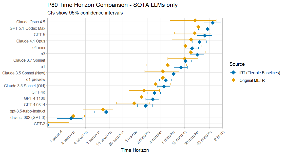
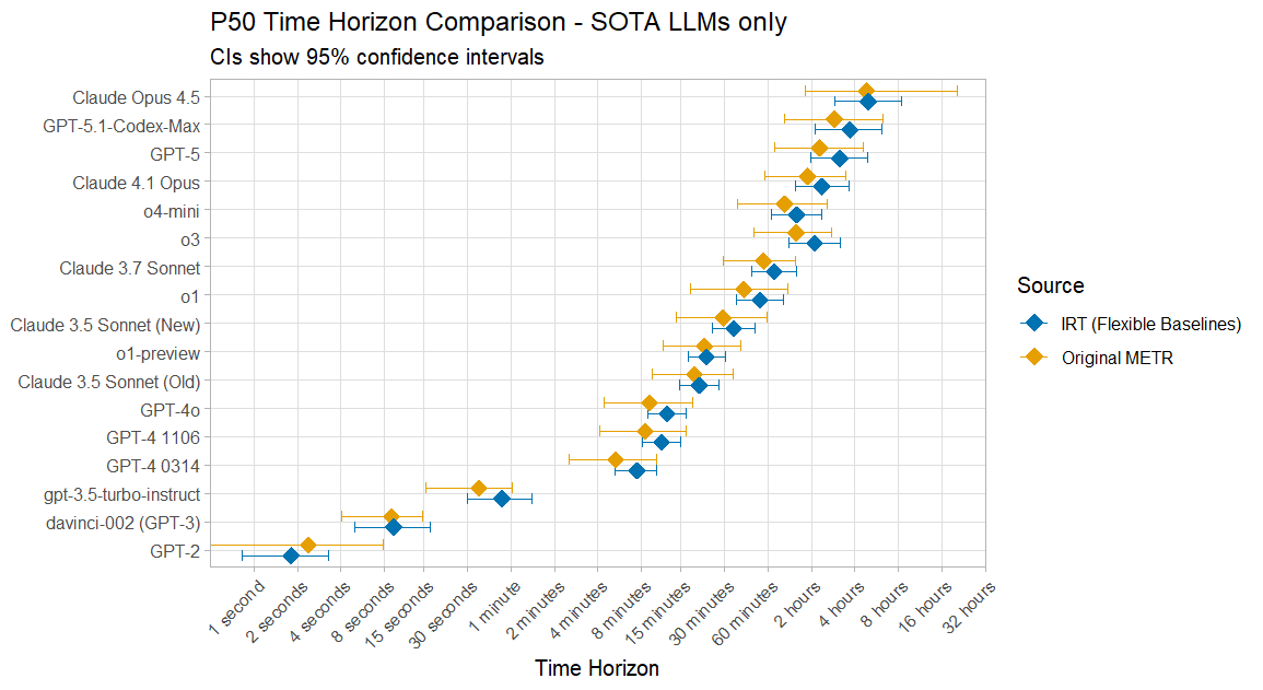
I think there is some natural increase due to how my model's data is selected however, as my 50% time horizons are also often somewhat higher, and they are mostly within uncertainty bounds anyway:
I've taken a very quick look through your code so try and think about the difference, and my guess would be that you find that LLM-difficulty diverges more from log(baseliner_time) time than I do, because you include the tasks with estimated baseliner times when calculating the amount of noise here, whereas I handled tasks with/without baseliner times separately, and only used the former when doing the time horizon calculations.
My definition was: "For a LLM m, I define its ‘p time horizon’ as the delta such that LLM m has (expected) probability p of success on a single attempt at a task with baseliner time delta." Where we might expect different results for tasks with estimated instead of baselined task lengths because there is effectively another layer of noise added by the estimates.
(I'll note that out of all the critiques of the Time Horizon work I'm surprised I don't see more discussion of the tasks which only have estimates, as this seems like one of the most straightforward limitations, and which will only get more relevant as tasks get longer and harder to baseline. Something like only 5/30 of the longest tasks currently have baseliner times!)
I've love to chat more about Bayesian modelling and general thinking about these kinds of models sometime, and thanks again for the interesting analysis.
However my 80% results ended up only being a factor of 2 lower than the results of METR's current model.
Aren't these a factor of 2 higher than the original METR model?
Good catch! Edited my comment. It had been a while since I had looked at the results and I must have also lost the ability to read in the meantime.
Very nice! I'm not able to comment very much since I don't know the specifics of your model, but can you clarify what you mean by
because you include the tasks with estimated baseliner times when calculating the amount of noise here, whereas I handled tasks with/without baseliner times separately, and only used the former when doing the time horizon calculations.
I have to admit I have worked with the METR data mostly as-is, and not gone into detail about how the times have been estimated. I suppose the problem is that only a subset of the tasks have grounded estimates of human times (as I interpreted HCAST?) and the rest are inferred in a more or less ad-hoc way? If so, then that would explain 80% marginal times being shorter because the residuals would (plausibly) be smaller.
Yes sorry for just dropping in with "I have a model that gives different results" without actually giving the details. I'm trying to get a minimal version of it written up (I had designed it to integrate into METR's codebase so need to extract it as something that can exits standalone).
Within the runs.json there is a (not especially clearly named) 'human_source' field for each row. If this is set to "baseline" then the task length is based on (one or more) human baseliners, if it is "estimate" then it was just estimated without any human actually finishing the task. These estimates are generally quite noisy - I believe somebody told me something like that for some of the tasks where they had both the estimates and the baseliner times, only 60% of the estimates were within a factor of 3 of the (average) baseliner times.
Because you have a unified sigma parameter for how difficulty-for-LLM differs from log(task_length) this ends up incorporating the estimate noise as an additional source of uncertainty. But if you define the p-time-horizon as I did in my first comment as being defined on baselined tasks only then these lead to different results for the 80% time horizons.
Update: Added GPT-5.2 to the main part of the text, this uses all data from v1.1. Added appendix using all METR models, by joining v1.0 and v1.1. Added appendix with marginal vs typical P(success) curves. Thanks to Thomas Kwa for telling me about this.
TLDR
I reanalyzed the METR task data using a Bayesian item response theory model.
METR data
Let’s start with a plot that shouldn’t be too surprising. Four reasonable models fit the METR data (v 1.1) equally well. They agree about the past but disagree strongly about the future.
The model selection scores known as ELPD-LOO differ by at most ~6 points. [1] Calibration is nearly identical, with Brier
These curves are fitted using a Bayesian item response theory model described below. Before describing it, let’s recall METR’s analysis of the time horizon. They proceed in two stages:
Per-model logistic regression. For each model
An OLS trend. Regress
This is good modeling and gets the main story right, but there are some non-standard choices here. For instance, the slope
In this post I make a joint model, adjust some things to be more in line with standard practice, and ask what happens when you try different trajectory shapes. The post is somewhat technical, but not so god-awful that Claude won’t be able to answer any question you have about the methodology. Models are fitted with Stan, 4 chains
The basic model
The first stage of METR’s model is almost a 2-parameter logistic model (2PL), the workhorse of educational testing since the 1960s.
So, what kind of problems was the 2PL model designed for? Say you give 200 students a math exam with 50 questions and record their answers as correct / incorrect. You want to estimate the students’ math ability, but raw percent correct scores aren’t necessarily very good, as they depend on which questions (easy or hard? relative to which students?) happened to be on the exam.
The 2PL model solves this by giving each student a single ability score (
The model estimates all parameters simultaneously via a logistic regression:
This matters here because METR tasks are like exam questions. They vary in both difficulty and how well they separate strong from weak models, and we want to put all the models on a common ability scale.
Modeling difficulty
Ability and difficulty parameters
Each task’s difficulty has a mean that depends on log human time, plus a random component to account for the fact that same-length tasks are not born equal. (METR treats all tasks of identical length as equally hard.)
Since difficulty increases with log human time at rate
I estimate
Of course, this is a modeling choice that can be wrong. There’s no guarantee that difficulty is linear in
A plotted dot at 5x means the task’s equivalent difficulty time is 5x its actual human time. Even within the
There’s not too much curvature in the relationship between log human time and difficulty, so I think the log-linear form is decent, but it’s much more spread out than we’d like. There is a cluster of easy outliers on the far left, which I think can be explained by very short tasks containing virtually no information about difficulty. Overall this looks reasonable for modeling purposes.
Modeling ability over time
By directly modeling ability over time, we can try out shapes like exponential, subexponential, superexponential, saturating, and singularity. Forecasts depend a lot on which shape you pick, and the data doesn’t really tell you much, so it’s not easy to choose between them. Your priors rule here.
The abilities are modeled as
where
If METR’s GitHub repo contained all the historical data, I would also have tried a piecewise linear with a breakpoint around the time of o1, which visually fits the original METR graphs better than a plain linear fit. But since the available data doesn’t go that far back, I don’t need to, and the value of including those early points in a forecasting exercise is questionable anyway. Getting hold of the latest data points is more important. (Added: I use all the data in the appendix below, but I do not attempt a piecewise linear since running the STAN programs take a lot of time.)
All models share the same 2PL likelihood and task parameters (
Each model except the saturating model will cross any threshold given enough time. Here are posteriors for the 50% crossing across our models. The saturating model almost never crosses the 1-month and 125-year thresholds since it saturates too fast.
Problems with 80% success
Everything above uses 50% success, but METR also cares about 80% success and fits a separate model for that. We don’t need to do that here since the model estimation doesn’t really depend on success rates at all. We’ll just calculate the 80%-success horizon using posterior draws instead.
But there are actually two reasonable ways to define “80% success,” and they give different answers.
Typical: Pick a task of average difficulty for its length. Can the model solve it 80% of the time? This is roughly what METR computes.
Marginal: Pick a random task of that length. What’s the expected success rate? Because some tasks are much harder than average, the hard ones drag down the average more than easy ones push it up.
At 50%, the two definitions agree exactly. But at 80%, the gap is roughly an order of magnitude!
So, on the one hand, it’s the variance (
The marginal horizon is the one that matters for practical purposes. “Typical” is optimistic since it only considers tasks of average difficulty for their length. The marginal accounts for the full spread of tasks, so it’s what you actually care about when predicting success on a random task of some length. That said, from the plot we see frontier performance of roughly 6 minutes, which does sound sort of short to me. I’m used to LLMs roughly one-shotting longer tasks than that, but it usually takes some iterations to get it just right. Getting the context and subtle intentions right on the first try is hard, so I’m willing to believe this estimate is reasonable.
Anyway, the predicted crossing dates at 80% success are below. First, the 1-month threshold (saturating model omitted since it almost never crosses):
And the 125-year threshold:
Make of this what you will, but let’s go through one scenario. Let’s say I’m a believer in superexponential models with no preference between quadratic and power-law, so I have 50-50 weighting on those. Suppose also I believe that 125 years is the magic number for the auto-coder of AI Futures, but I prefer
Let’s also have a look at METR’s actual numbers. They report an 80% horizon of around 15 minutes for Claude 3.7 Sonnet (in the original paper). Our typical 80% horizon for that model under the linear model is about 21.1 min, and the marginal is about 0.8 min, roughly 15x shorter than METR’s.
Modeling
The available METR data contains the geometric mean of (typically 2-3 for HCAST) successful human baselines per task, but not the individual times. Both METR’s analysis and mine treat this reported mean as a known quantity, discarding uncertainty. But we can model
I’d expect smaller differences between the typical and marginal plots at
A technical point: When modeling
Notes and remarks
Appendix: Results for all models
Recall that the main text uses only METR v1.1 data. In this appendix I use all available data (v1.0 + v1.1 merged). The overall story is similar, but the pre-Sonnet-3.5 models introduce a visible kink in the trajectory that a single smooth trend struggles with. (This is well-known.)
The ELPD-LOO scores differ by at most ~3 points, with Brier
Appendix: Marginal vs typical success curves
These are fitted on v1.1 data only.
The ELPD-LOO estimates are: power-law
Define
The multiplier is
Quadratic is the simplest choice of superexponential function. You could spin a story in its favor, but using it is somewhat arbitrary. The power-law is the simplest function that can be both super- and subexponential (in practice turns out to be superexponential here though), and I included the saturating model because, well, why not? ↩︎
The ELPD-LOO estimates are: power-law