Functional form

Bayes's Rule generalizes to continuous functions, and states, "The posterior probability density is proportional to the likelihood function times the prior probability density."

$P(H_x\mid e)\propto L(e\mid H_x)\cdot P\left(H_x\right)$

Example

Suppose we have a biased coin with an unknown likelihood $f$ between 0 and 1 of coming up heads on each individual coinflip. Since the bias $f$ is a continuous variable, we express our beliefs about the coin's bias using a probability density function that gives the chance for the coin's bias $f$ to be found inside a tiny interval $df.$

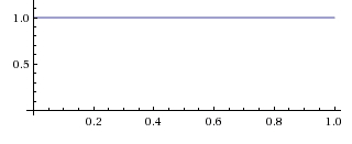
By hypothesis, we start out completely ignorant of the bias $f,$ meaning that all initial values for $f$ are equally likely. $P\left(f\right)=1$ or $P\left(f\right)df=1\cdot df.$ (E.g., the chance of $f$ being found in the interval from 0.91 to 0.92 is 0.01.)

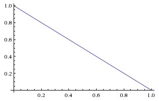
We then flip the coin, and observe it to come up tails as our first piece of evidence. This observation $e_1=\text{T}$ has a likelihood $L(e_1=\text{T}\mid f)$ of 0.4 if the bias $f$ is 60% heads, a likelihood of 0.67 if $f=0.33,$ etcetera.

Graphing the likelihood function $L(e_1=\text{T}\mid f)$ as it takes in the fixed evidence $\text{T}$ and ranges over variable $f,$ we obtain the straightforward graph $L(e_1=\text{T}\mid f)=1-f.$

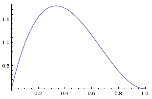
If we multiply the likelihood function by the prior probability function as it ranges over $f$, we obtain a relative probability function on the posterior, $O(f\mid e_1=\text{T})=L(e_1=\text{T}\mid f)\cdot P\left(f\right)=1-f,$ which of course looks just like:

But this can't be our posterior probability function because it doesn't integrate to 1. ${\int }_0^1(1-f)df=\frac{1}{2}.$ (The area under a triangle is half the base times the height.) Normalizing this relative probability function will give us the posterior probability function:

$P(f\mid e_1=\text{T})=\frac{O(f\mid e_1=\text{T})}{{\int }_0^{1}O(f\mid e_1=\text{T})df}=2\cdot (1-f)$

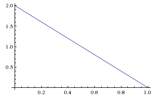
The shapes are the same, and only the y-axis labels have changed to reflect the different heights of the pre-normalized and normalized function

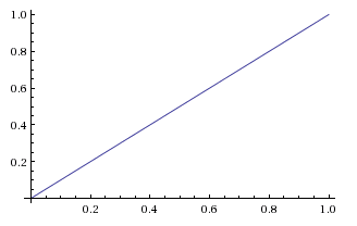
Suppose we now flip the coin another two times, and obtain the next piece of evidence, $e_{2,3}=\text{HT}.$ Although these two pieces of evidence pull in opposite directions with respect to any particular value of $f,$ they don't cancel out as net evidence about every possible bias; they don't pull with the same strength on all possibilities for $f.$ If we see $\text{HT}$ then this has probability $0$ if $f=0,$ so seeing this entirely rules out that the coin is all-tails.

We multiply the old belief

by the additional pieces of evidence

and

and obtain the posterior relative density

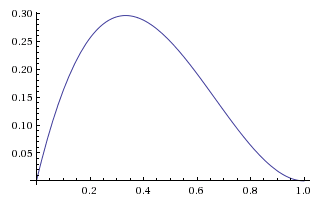
which is proportional to the normalized posterior probability

Or, writing out the whole operation from scratch:

$P(f\mid e=\text{THT})=\frac{L(e=\text{THT}\mid f)\cdot P\left(f\right)}{P(e=\text{THT})}=\frac{(1-x)\cdot x\cdot (1-x)\cdot 1}{{\int }_0^1(1-x)\cdot x\cdot (1-x)\cdot 1df}=12\cdot f(1-f{)}^2$

Note that it's okay for a posterior probability density to be greater than 1, so long as the total probability mass isn't greater than 1. If there's probability density 1.2 over an interval of 0.1, that's only a probability of 0.12 for the true value to be found in that interval.

Note also that there's no reason to normalize likelihood functions, and it would be meaningless to do so. There's no reason for the probability of seeing $\text{THT},$ summed over each of the possible $f,$ to sum to $1$ a priori.