For the toy model, I'd like it if you explicitly showed that there are inputs on which the CLT replacement model gives very different outputs to the original model. You could then check whether the PLT replacement model performs better than the CLT one on these inputs. This result should be simple to obtain: just choose a nonbinary input, i.e. an that is not in . But it would make the toy model more compelling to me, since, to me, faithfulness is really about OOD generalization.
Thanks for your thoughtful comment! I think that's an interesting idea. If a replacement model is faithful, you would indeed expect it to behave similar when tested on other data. This may possibly connect to a related finding that we couldn't yet explain: that CLTs fail for memorized sequences, when those should be the simplest. Maybe the OOD test is something that we could do in real LLMs as well, not just toy models.
I don't think I'd go as far as saying "faithfulness==OOD generalization" though. I think it is possible that two different circuits produce the same behavior, even on OOD. For example, let model A and B learn to multiplicate arbitrary numbers perfectly. There are different ways to do x * y, for example compute +x y times, do it like we learned in school, etc. In those cases, OOD examples would still deliver equal output but the internal circuits are different. So I'd say that faithfulness is a stronger claim than OOD generalization.
I won't argue about definitions of faithfulness - yours seems as fine as any - but I think I only care about unfaithfulness in as far as it causes our circuits to make incorrect predictions about OOD behavior.
One data point on the proposed mitigations: I experimented a little with summed per-layer L2 norms for the decoder norms in the sparsity penalty while training CLTs for Qwen 3 and didn't see much difference in the spread of per-layer L0. It did result in a bigger range of decoder norms and hence effective feature activation magnitudes, which made calibrating the coefficient inside the tanh more difficult. It may be that another loss term directly penalizing decoder norms would help here.
Great post! Two thoughts I had:
(a) (echoing jacob_drori's point) I'm not sure about your specific trained CLT, but I believe it is possible to construct a faithful one-layer CLT in this task (you could do everything with a MLP!). In this case, does it really matter if we are observing the circuit?
(b) I think the contribution plot is very compelling, but the case study isn't very convincing to me as another way to phrase it seems to be "CLT missed the middle-layer feature in this particular case".
Thanks for your comment, I really appreciate it!
(a) I claim we cannot construct a faithful one-layer CLT because the real circuit contains two separate steps! What we can do (and we kinda did) is to have a one-layer CLT to have perfect reconstruction always and everywhere. But the point of a CLT is NOT to have perfect reconstruction - it's to teach us how the original model solved the task.
(b) I think that's the point of our post! That CLTs miss middle-layer features. And that this is not a one-off error but that the sparsity loss function incentivizes solutions that miss middle-layer features. We are working on adding more case studies to make this claim more robust.
Many thanks to Michael Hanna and Joshua Batson for useful feedback and discussion. Kat Dearstyne and Kamal Maher conducted experiments during the SPAR Fall 2025 Cohort.
TL;DR
Cross-layer transcoders (CLTs) enable circuit tracing that can extract high-level mechanistic explanations for arbitrary prompts and are emerging as general-purpose infrastructure for mechanistic interpretability. Because these tools operate at a relatively low level, their outputs are often treated as reliable descriptions of what a model is doing, not just predictive approximations. We therefore ask: when are CLT-derived circuits faithful to the model’s true internal computation?
In a Boolean toy model with known ground truth, we show a specific unfaithfulness mode: CLTs can rewrite deep multi-hop circuits into sums of shallow single-hop circuits, yielding explanations that match behavior while obscuring the actual computational pathway. Moreover, we find that widely used sparsity penalties can incentivize this rewrite, pushing CLTs toward unfaithful decompositions. We then provide preliminary evidence that similar discrepancies arise in real language models, where per-layer transcoders and cross-layer transcoders sometimes imply sharply different circuit-level interpretations for the same behavior. Our results clarify a limitation of CLT-based circuit tracing and motivate care in how sparsity and interpretability objectives are chosen.
Introduction
In this one-week research sprint, we explored whether circuits based on Cross-Layer Transcoders (CLTs) are faithful to ground-truth model computations. We demonstrate that CLTs learn features that skip over computation that occurs inside of models. To be concrete, if features in set A create features in set B, and then these same set B features create features in set C, CLT circuits can incorrectly show that set A features create set C features and that set B features do not create set C features, ultimately skipping B features altogether.
This matters most when researchers are trying to understand how a model arrives at an answer, not just that it arrives at the correct answer. For instance, suppose we want to verify that a model answering a math problem actually performs intermediate calculations rather than pattern-matching to memorize answers, or detect whether a model's stated chain-of-thought reasoning actually reflects its internal computation. If CLTs systematically collapse multi-step reasoning into shallow input-output mappings, they cannot help us distinguish genuine reasoning from sophisticated lookup - precisely the distinction that matters for both reliability and existential risk. A model that merely memorizes may fail unpredictably on novel inputs; a model that reasons deceptively may actively conceal its true objectives. Interpretability tools that skip over intermediate computation cannot help us tell the difference.
We demonstrate the “feature skipping” behavior of CLTs on a toy model where ground-truth features are known, showing that the CLT loss function biases models toward this behavior. We then present evidence that this phenomenon also occurs in real language models.
Background
The goal of ambitious mechanistic interpretability is to reverse engineer an AI model’s computation for arbitrary prompts and to understand the model's internal neural circuits that implement its behavior. We do this in two steps: first, we discover which features are represented at any location in the model. Second, we trace the interactions between those features to create an interpretable computational graph.
How? The primary hypothesis in mechanistic interpretability is that features are represented as linear directions in representation space. However, there are more features than there are model dimensions, leading to superposition.
Sparse dictionary learning methods like sparse autoencoders (SAEs, link and link) can disentangle dense representations into a sparse, interpretable feature basis. However, we cannot use SAEs for circuit analysis because SAE features are linear decompositions of activations, while the next MLP applies neuron-wise nonlinearities, so tracing how one SAE feature drives another requires messy, input-dependent Jacobians and quickly loses sparsity and interpretability. Transcoders, on the other hand, are similar to SAEs but take the MLP input and directly predict the MLP output using a sparse, feature-based intermediate representation, making feature-to-feature interactions inside the MLP easier to track. When we train transcoders for every layer, we can trace circuits by following feature interactions between these transcoders rather than inside the original network, effectively replacing each MLP with its transcoder and turning the whole system into a “replacement model”. Crucially, the resulting circuits are technically part of the replacement model, which we simply assume are an accurate representation of the base model.
However, it has been observed that similar features activate across multiple layers, which makes circuits very large and complex. It is hypothesized that this is due to cross-layer superposition, where multiple subsequent layers act as one giant MLP and compute a feature in tandem. To learn those features only once, and thus reduce circuit size, Anthropic suggested cross-layer transcoders (CLTs).
A cross-layer transcoder is a single unified model where each layer has an encoder, but features can write to all downstream layers via separate decoders: a feature encoded at layer ℓ has decoder weights for layers ℓ, ℓ+1, ..., L. Crucially, following Anthropic's approach, all encoders and decoders are trained jointly against a combined reconstruction and sparsity loss summed across all layers. The sparsity penalty encourages features to activate rarely, which, combined with cross-layer decoding, pushes features to span multiple layers of computation. Anthropic found this useful for collapsing redundant "amplification chains" into single features and producing cleaner attribution graphs.
Here, we show that this same property can cause CLTs to skip over intermediate computational steps that occur in the original model and therefore create an unfaithful representation of the model’s computation. We call a circuit representation faithful if it captures the actual computational steps the model performs, that is, if the features it identifies as causally relevant match the intermediate computations that would be revealed by ablating the corresponding model components. This extends previous findings that show PLTs can be unfaithful.
Crosslayer Superposition vs Multi-step Circuits
Figure 1: Distinction between crosslayer superposition and multi-step circuits (modified from Anthropic’s paper)
The motivation for using cross-layer transcoders is to represent features that are computed in superposition across multiple subsequent layers only once. But how do we decide whether multiple subsequent layers are computing a single feature in cross-layer superposition, versus implementing a multi-step circuit that should be represented as two or more distinct features at different layers?
We draw the distinction as follows. In Anthropic’s framing, cross-layer superposition occurs when several consecutive layers effectively act like one large MLP (see figure). In this case, there is no meaningful intermediate interaction between layers for that feature and the layers contribute additively and reinforce the same feature direction. By contrast, we say the model is implementing a multi-step circuit when the computation relies on intermediate features that are computed in one layer and then used by a later layer, for example when layer A computes a feature that is then read and transformed by layer B into a new feature (right-most panel of Figure 1).
A simple diagnostic is whether the intermediate feature lives in a different subspace. If layer A writes to a direction that is largely orthogonal to the feature that layer B outputs, then layer A is not merely amplifying the same feature across layers. Instead, layer A is computing a distinct intermediate feature that layer B later transforms, which is unambiguous evidence of a multi-step circuit rather than cross-layer superposition.
Here, we show that the same mechanism that enables CLTs to capture cross-layer superposition can also cause them to approximate a genuine multi-step circuit as a single-step circuit, producing a circuit that differs from the model’s true intermediate computations and is therefore unfaithful.
CLTs Are Not Faithful in a Toy Model
In this section, we construct a toy model computing boolean functions. We manually set weights that implement a two-step algorithm which serves as a ground truth circuit. We then train PLTs and CLTs and show that CLTs learn two parallel single-hop circuits, thus being unfaithful to the ground truth.
Toy Model Overview
We handcrafted a toy model to compute the boolean function (a XOR b) AND (c XOR d), with four binary inputs (+1 or -1). The model has two MLP-only layers with residual connections.
Layer 0 has four neurons computing the partial products needed for XOR: ReLU(a - b - 1), ReLU(b - a - 1), ReLU(c - d - 1), and ReLU(d - c - 1). We call these outputs e, f, g, h. Layer 1 computes i = ReLU(e + f + g + h - 1), which is true if and only if both XORs are true.
Each of these nine values (four inputs, four intermediate features, one output) occupies its own linear subspace in the residual stream.
Figure 2: We construct a toy model implementing the Boolean function: (a XOR b) AND (c XOR d) using a 2-layer residual MLP.
Cross-Layer Transcoder Training
We collect MLP input and output activations for all 16 possible inputs and train a JumpReLU cross-layer transcoder with 32 features per layer until convergence following Anthropic’s approach. Since our model has two layers, the CLT trains two separate sets of features. The first set encodes the four inputs to the model (the mlp_in) and outputs two separate decoders to predict the output of neurons, also shown in Figure 3: one decoder predicts the output of the layer-0 neurons and the other predicts the output of the layer-1 neuron. For the second set of features, the encoder takes in the residual stream after the first MLP (namely the model inputs and the outputs of the first MLP) and decodes to match the output of the second MLP. Importantly, we standardize input and output activations to ensure that reconstruction errors are weighted equally across layers.
The CLT Skips Intermediate Computation
Figure 3: Left: The original ground truth residual MLP that learned a 2-step circuit A -> B -> C. Right: The crosslayer transcoder that learned to approximate the original model by learning two one-step circuits A -> **B (**correct) and A -> **C (**incorrect).
We trained CLTs with varying sparsity penalties and found perfect reconstruction even with an average L0 loss of ~1.0 per layer. We find that with sufficient sparsity pressure and enough features, the CLT learns to not activate any layer-1 features at all but still recovers second layer output perfectly via the first layer’s second decoder (see Figure 3 and Table 1). We can directly read off this behavior from the CLT’s weights (see Appendix). Both PLT and CLT achieve perfect reconstruction accuracy but the CLT never activates any features in layer 1. Instead, it uses more features in layer 0 and directly constructs layer 1 output, effectively creating a single-hop circuit that directly maps the input to output.
But from how we defined our model, we know that this does not match our model’s true internal algorithm. The single neuron in layer 1 is performing important computation on existing intermediate results to determine if the boolean expression is true. If we ablate this neuron, nothing writes to the output channel i, and the network cannot determine the value of the overall boolean expression. The CLT suggests that both MLPs learned features in crosslayer superposition but this is importantly not the case here: We can show by ablating the interaction between MLP 0 and MLP 1 (which in our case is trivially easy because they occupy their own linear subspace) that this breaks the model. Therefore, the CLT learned an unfaithful circuit.
This alone is all we need to argue that the CLT is not faithful. The post-mlp0 features are responsible for the post-mlp1 feature. Our CLT fails to capture this.
Table 1: Core metrics of JumpReLU CLT vs PLT.
Other Results
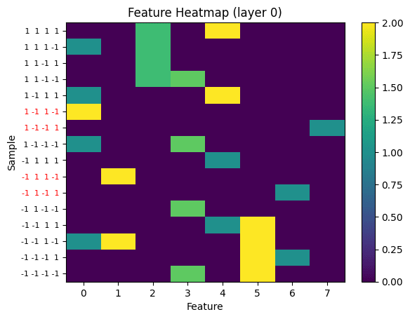
Despite missing the second layer's computation, the CLT still reconstructs the full residual stream accurately. It learns 8 alive features that function as a lookup table: four features (0, 4, 13, 14) correspond to the four input combinations where the overall expression is TRUE, directly setting all intermediate and final outputs. The other four alive features (6, 7, 9, 11) each detect when one XOR is FALSE and zero out the corresponding intermediate features.
While this lookup table correctly computes all outputs, it does not reflect how the model actually performs computation step-by-step. We could implement the same boolean function with a 1-layer MLP using just these four "TRUE-case" features—but that is not the model we trained, which is why we argue the CLT is unfaithful.
Figure 4: Jump-ReLU CLT features
The CLT’s Loss Function Incentivizes this Bias
Our toy model demonstrates that CLTs can learn unfaithful representations, but one might wonder whether this actually occurs in practice on real language models. Proving that CLTs learn unfaithful circuits for frontier LLMs is challenging because we don’t have ground truth circuits that we could compare against. Instead, in this section, we first make a theoretical argument on how the sparsity objective may bias the CLT towards learning shorter but unfaithful circuits and then test predictions of this hypothesis in GPT-2 and Gemma 2.
Intuition
Why are CLTs capable of learning unfaithful circuits in the first place? Deep neural computations can often be approximated by much shallower networks, by the universal approximation theorem. A CLT effectively gives us a sparse, giant shallow MLP: early-layer features can directly write to many downstream layers via their decoders, so the replacement model has an easy path to represent deep computations as shallow input-output mappings.
A natural objection is that shallow approximations typically require many more neurons, which should push the CLT toward learning the true intermediate structure instead of shortcutting it. That is true in principle, but it misses a key asymmetry in CLTs: additional decoder vectors are almost free. The CLT needs to encode features starting at layer 0 - meaning there are active features that encode and decode in layer 0; once a feature is already active, giving it additional decoder vectors to multiple later layers does not meaningfully increase the sparsity loss. As a result, we should expect at least some amount of depth collapse: the CLT can move a significant fraction of computation into early features.
A second objection is that this “free decoder” argument only holds for TopK CLTs, since JumpReLU or ReLU CLTs also penalize decoder norms. But even there, additional decoder vectors remain close to free: because the penalty is applied to the concatenated decoder vector rather than separately per layer, spreading mass across many decoders increases the norm only sublinearly. In practice, using extra decoder vectors costs far less than activating additional features in later layers, so the shortcut representation can still dominate.
Overall, the CLT objective is indifferent to faithfulness: it rewards reconstruction accuracy and sparsity, not preserving intermediate computational steps. When a shallow shortcut matches reconstruction while paying less sparsity cost than a layered decomposition, the CLT is incentivized to learn the shortcut.
Evidence from Real Language Models
We next test predictions of the above theory. First, we show that CLTs shift L0 towards earlier layers compared to PLTs. Second, we show that attribution circuits on natural text are much more dependent on earlier layers.
Asymmetric L0 Across Layers
We train JumpReLU CLTs and PLTs on gpt2-small and use Anthropic’s method except where specified otherwise. We train on 100M tokens with a batch size of 1000 on the OpenWebText dataset. We collect and shuffle activations from gpt2-small and standardize both input and output activations. We train with 10k features per layer and tune L0 to be around 12-15 active features per layer.
To check that the low L0 in later layers is not simply an artifact of layer-specific activation geometry, we train Per-Layer Transcoders (PLTs) under an otherwise matched setup. Crucially, unlike approaches that train each layer independently, we sum the loss across all layers and train all layers jointly. If a non-uniform L0 profile were driven by the inherent structure of the activations, we would expect the same pattern to appear for PLTs.
Instead, we find that only CLTs show a strong asymmetry: layer 0 has much higher L0 than later layers, often more than 3× higher, with late layers especially sparse (left panel in Figure 5). This pattern is not explained by activation geometry. When we train PLTs jointly, L0 remains similar across layers (right panel). The asymmetry appears only for CLTs, matching our theoretical prediction: early-layer features do disproportionate work because they can write to all downstream layers at little additional cost.
Figure 5: L0 for JumpReLU CLT (left) and PLT (right) trained on GPT2-small and OpenWebText.
CLT Circuits Attribute to Earlier Layers
Here, we show that attribution circuits computed with CLTs rely heavily on early layers whereas attribution for PLTs is linear. For our experiments, we used Gemma2-2b as our base model, the Cross-Layer Transcoder from Hanna & Piotrowski (CLT-HP) as the CLT, and Gemmascope-2b Transcoder as the PLT. We ran 60 prompts through the replacement model of both the PLT and CLT. These prompts consisted of an equal split of memorized sequences (e.g., MIT license), manually constructed prompts, and random sentences from the internet (e.g., news articles and Wikipedia). From these graphs, we computed the fraction of total contribution to the top output logit (the model's highest-probability prediction) from features in layers 0 through n. Specifically, we collected all positive-weight edges in the attribution circuit and calculated:
where El is the set of edges from features in layer l and we is the weight of edge e.
By repeating this calculation for increasing values of n (from 0 to the total number of layers), we generated cumulative contribution curves showing what proportion of total attribution comes from early layers at each depth. Figure 6 shows that, for the PLT, all layers contribute comparably, and the cumulative circuit contribution grows roughly linearly with depth. In contrast, the CLT exhibits a sharp jump at layer 1, with nearly all contributions concentrated in layers 0 and 1.
Figure 6: We compute attribution circuits on 45 prompts and compute layerwise cumulative contribution to circuits that compute the largest output logit.
Together, these results are consistent with our theory: CLTs concentrate both sparsity budget and attribution mass in early layers, while PLTs distribute contribution more evenly across depth, suggesting partial depth collapse in CLT replacement circuits. This is only indirect evidence, though, since we do not have ground-truth circuits in real LLMs and cannot directly test faithfulness the way we can in the toy model.
Divergent Circuit Interpretations: License Memorization
Finally, we show that “CLTs in the wild” can produce wildly different high-level conclusions. Specifically, we show an “existence proof” of some abstract features that activate on diverse prompts and are steerable but don’t exist in the CLT. Then, we investigate mechanisms of memorization and generalization in software licenses and show that interpreting CLTs would lead to different conclusions.
In the Wild: A Real Feature the CLT Doesn’t Learn
We examined verbatim memorization of the MIT license in Gemma-2-2B, specifically the prediction of " sell" after the phrase "publish, distribute, sublicense, and/or." We want to understand whether memorized and generalized circuits interact or collaborate, or whether verbatim memorization elicits completely different circuits compared to generalization.
Using PLTs, we find two important groups of features (a.k.a. supernodes) in late layers at the “ or” position: Output features that when active push logits for any form of the word sell (e.g. “ sell”, “ sold”, “ selling”, “ sale”; Neuronpedia) and features that activate on lists of present-tense verbs and push logits for present-tense verbs (e.g. “ edit”, “ build”, “ install”, “ sell”, “ fill”, “ move”, “ bake”; Neuronpedia). Together, they positively interfere to push the (memorized) “ sell” token to ~100%.
The latter features’ max-activating examples contain text from diverse contexts and can reliably be activated: We LLM-generate 20 prompts that contain lists of present-tense verbs and 20 controls. 11/20 prompts activated the features at the expected positions while the features fired for none of the controls. Steering those features with modest strength (-0.7x) makes the model predict “ selling” instead of “ sell” (Figure 7).
Crucially, this works on arbitrary text and is not specific to MIT license memorization. We hand-write a new non-existent license text that loosely mirrors some characteristics (specifically, it also contains a list of present tense verbs). On this prompt, the same supernode is active, and steering yields similar results: It pushes the output distribution from present-tense to the participle (i.e. “ publishing”, “ printing”, “ licensing”; Figure 7).
Figure 7: Steering feature L22::14442 and L25::9619 on the MIT license and a similar but made-up license.
We investigated CLT circuits (Figure 9) for this prompt but could not find any counterpart to this supernode. It would only be defensible for the CLT to “absorb” this intermediate feature into an upstream MIT license memorization feature if the intermediate feature were itself license specific, meaning it reliably fired only in memorization contexts. But these PLT features are clean, monosemantic, and causally steerable across diverse prompts, including both memorized and non-memorized sequences. Since they implement a general present tense verb to participle transformation that applies far beyond the MIT license, collapsing them into a license memorization circuit erases a real intermediate computation that the base model appears to use and should therefore be represented as its own feature.
How CLTs Lead to the Wrong Story
What is the downstream consequence? We now build and interpret the full circuit graph for the MIT license continuation and show that the CLT and PLT lead to qualitatively different mechanistic stories about what the model is doing.
The CLT graph suggests a lookup-table-like memorization mechanism with little reuse of general language circuitry, while the PLT graph supports a different picture where general present tense verb circuitry (and others) remains intact and memorization appears as a targeted correction on top:
PLT Interpretation: Generalization with minimal memorization (see Figure 8) In the PLT, the next token prediction emerges from two interacting circuits: one promoting "sale-words" and another promoting "present-tense verbs," which together predict "sell" with approximately 100% probability. The present-tense-verb feature directly connects to the embeddings of the present-tense verbs in the list and some software/legal context features. The "sale-words" feature is activated by a larger abstract circuit that first recognizes the "and/or" construction and separately the software-licenses context. There are also direct connections from MIT-license-specific token embeddings to the "say sell-words" feature, which may represent a memorization mechanism. Our interpretation with PLTs is that the model's generalized circuits are always active, with a few lookup-table features that encode the difference between the generalized logits and the actual memorized logits.
Figure 8: PLT circuit for MIT license memorization.
CLT Interpretation: Pure memorization (see Figure 9) For the CLT, we also find an important "say sell-words" feature and a feature that fires at exactly all commas in this MIT verb enumeration. However, these features primarily connect directly to layer-0 and layer-1 features. These early features encode either token identity or fire unconditionally (high-frequency features). The CLT interpretation suggests the circuit is completely memorized without generalized circuits that interact and collaborate.
Figure 9: CLT circuit for MIT license memorization.
These are not minor differences in circuit topology; rather, they represent fundamentally different theories of how the model performs this task. If the PLT interpretation is correct, the model has learned a generalizable linguistic structure that it applies to memorized content. If the CLT interpretation is correct, the model simply pattern-matches to memorized sequences. Understanding which is true matters for predicting model behavior on novel inputs, assessing robustness, and evaluating the degree to which models have learned generalizable concepts versus surface statistics.
Our theory explains this divergence. The CLT's bias toward early-layer features causes it to represent the computation as a shallow lookup from input tokens to outputs, collapsing away the intermediate abstract features that PLTs surface. The generalized circuits may not be absent from the model; they may simply be absent from the CLT's representation of the model.
Discussion
The Crosslayer Superposition Tradeoff
The original motivation for CLTs was handling crosslayer superposition, where the same concept appears redundantly across layers. Our findings reveal an uncomfortable tradeoff: the same mechanism that efficiently captures persistent features also enables skipping intermediate computations. A feature legitimately persisting from layer 0 to layer 10 can look identical to a shortcut that bypasses layers 1 through 9. This suggests that, under the current CLT architecture, faithfulness and efficient handling of crosslayer superposition may be fundamentally in tension.
This concern started from practice, not theory. We were excited about attribution circuits, used them heavily, and then noticed a consistent mismatch: results that looked robust with PLTs were often not replicable with CLTs, and the two tools sometimes implied very different circuit stories for the same prompts and behaviors. We also found that feature steering with CLTs was often less straightforward than we expected. Because CLTs represent features only once rather than redundantly across layers, we initially hoped steering would become easier, but we frequently observed the opposite. This does not prove unfaithfulness on its own, but it fits the broader pattern that CLT circuits can be harder to interpret and manipulate as if they were directly tracking the model’s intermediate computations.
Detection and Mitigation
Given the systematic bias toward unfaithfulness, practitioners need methods to detect and potentially correct this behavior.
Detection approaches
The most direct signal is asymmetric L0 across layers. If early layers show dramatically higher feature activation than late layers, computation is likely being collapsed into early features. Comparing CLT and PLT L0 distributions on the same model can reveal the extent of this collapse.
Researchers should also compare CLT-derived circuits against causal interventions. If ablating an intermediate neuron disrupts model outputs but the CLT shows no intermediate features contributing, this indicates unfaithfulness. A feature set with L0 of zero for a layer containing clearly active neurons is a particularly strong signal.
More specifically, to verify a claim of crosslayer superposition and rule out a genuine multi-step circuit, it is not enough to ablate a neuron in isolation. One must ablate the interaction between layers for the putative feature: if the computation truly reflects crosslayer superposition, then breaking the handoff between layers should not destroy the behavior, since the “same feature” is effectively being maintained across layers. If, instead, the behavior depends on intermediate information computed in one layer and transformed in a later layer, then ablating the inter-layer interaction should break the computation. This kind of targeted inter-layer ablation is the cleanest causal test distinguishing crosslayer superposition from multi-step circuits.
Finally, qualitative comparison between CLT and PLT circuits on the same computation can surface discrepancies warranting investigation, as in our memorization example.
Mitigation approaches
We have not yet systematically tested mitigations, but outline several directions based on our analysis:
Penalizing L0 asymmetry. One could add a regularization term discouraging extreme differences in feature activation across layers. However, this risks forcing spurious features when a layer genuinely performs minimal computation.
Separating decoder norm penalties. The most direct fix would modify the sparsity penalty to sum separate L2 norms for each layer's decoder, rather than computing the norm of the concatenated vector. This removes the geometric advantage we identified: using N decoder vectors would cost ~N rather than ~√N, matching the cost of separate features at each layer. We have not yet trained CLTs with this modification.
Limiting feature span. Architectural constraints could restrict how many layers a single feature can decode to, for example by using a sliding window of k downstream layers. This sacrifices some ability to represent genuine crosslayer superposition but forces multi-step computation to use multiple features. It would also make CLT training far less computationally intensive: instead of learning decoders for all layer pairs, which scales like n^2 in the number of layers n, you would learn only n⋅k decoders. In large models this can be a big win, for example n=80 but only allowing decoders to the next k=5 layers.
Auxiliary faithfulness losses. A more principled approach might reward features whose activations correlate with actual neuron activations at each layer, rather than only rewarding output reconstruction. This directly incentivizes tracking the model's internal states.
Local crosslayer transcoders**.** Another pragmatic mitigation is to restrict each feature’s decoder to only write to a local neighborhood of downstream layers, for example the next k=5 layers, instead of allowing writes to all later layers. This does not fundamentally remove the incentive to “collapse” multi-step computation, since a feature can still span multiple layers within its window and you can still chain windows. But it can plausibly fix the common case in practice: many of the problematic absorptions we see involve long range decoding where a single feature effectively jumps over intermediate computations. Enforcing locality makes it harder for the CLT to bypass those steps, and encourages the representation to expose intermediate features rather than compressing them away. This is an 80/20 style mitigation: it may not guarantee faithfulness, but it could substantially reduce the worst failures while also lowering training cost by replacing all pairs decoding with n⋅k decoders instead of n^2.
We consider the separated decoder norm penalty the most promising near-term experiment, as it directly addresses the cost asymmetry without requiring architectural changes or auxiliary objectives.
Limitations
Our primary demonstration uses an extremely small toy model that we hand-crafted to have known ground-truth features. This controlled setting allowed us to definitively identify unfaithfulness, but it may not be representative of computations in real language models.
Our primary demonstration uses an extremely small toy model with known ground-truth features. While this controlled setting allowed us to definitively identify unfaithfulness, the toy model's 16 possible inputs and simple boolean function may not be representative of real language models. In higher-dimensional settings, lookup-table shortcuts may be infeasible, forcing more compositional representations.
The evidence from Gemma-2-2B is suggestive but not definitive. Without ground truth for what computations the model actually performs, we cannot be certain which interpretation (CLTs or PLTs) is correct. It is possible that the model genuinely implements memorization via shallow lookup tables, and the CLT is faithfully representing this while the PLT invents spurious intermediate structure. Our theory predicts CLT unfaithfulness, but this particular case could be an instance where the CLT happens to be correct.
Finally, our analysis focused on MLPs and did not examine attention layers. Cross-layer transcoders spanning attention computations may exhibit different failure modes, as the computational structure of attention differs significantly from feedforward layers.
Conclusion
Cross-Layer Transcoders offer computational advantages over per-layer alternatives, particularly in handling crosslayer superposition. However, the same architectural properties that enable these advantages create a systematic bias toward unfaithful representations that collapse intermediate computations into shallow input-output mappings.
We demonstrated this unfaithfulness in a toy model where ground-truth features are known, explained the loss function dynamics that create this bias, and showed evidence that the phenomenon affects real language model interpretability - with meaningfully different conclusions about model behavior depending on which tool is used.
Understanding and mitigating this faithfulness problem is important for the field of mechanistic interpretability. We hope this work encourages both caution in interpreting CLT circuits and further research into training procedures that better balance efficiency and faithfulness.
Appendix
Contributions
Georg came up with the research question. Rick selected and handcrafted the model. Georg trained the CLTs on the handcrafted model. Rick and Georg interpreted these CLTs and wrote up the results. Georg conducted the experiments with real language models and wrote this section. Kamal and Kat conducted experiments for and wrote the “CLT Circuits Attribute to Earlier Layers“ section. Georg supervised Kamal and Kat through the SPAR AI program. Rick and Georg wrote the conclusion section. We jointly edited the writeup.
Full Analysis of JumpReLU CLT (L0=2)
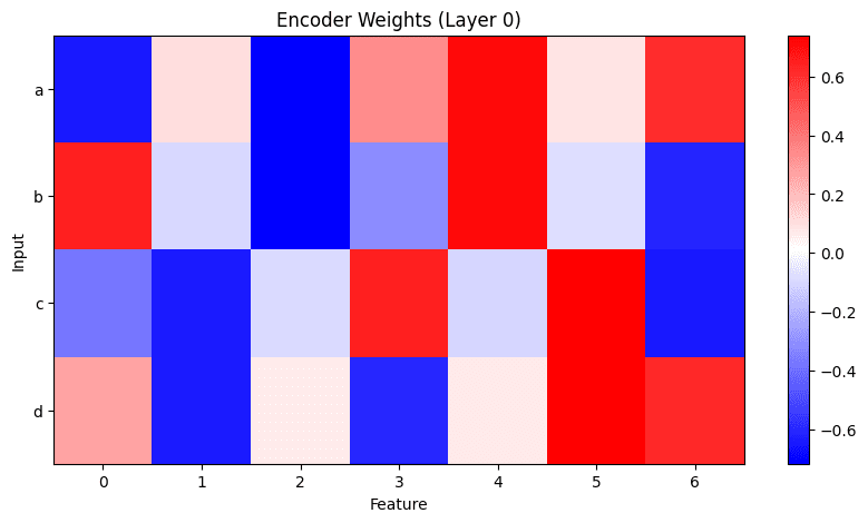
We train a JumpReLU CLT with 32 features and tune the sparsity coefficient to yield an L0 of 2 across both layers. The CLT learns to activate ~2 features in layer 0 and none in layer 1. In layer 0, 8 of the 32 features are alive. We only plot weights and activations of living features.
The encoder weights learn different combinations of input features:
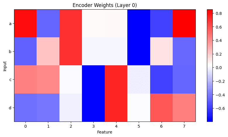
One feature is active for the inputs that should output 1, and two or three features are active for inputs that should output -1.
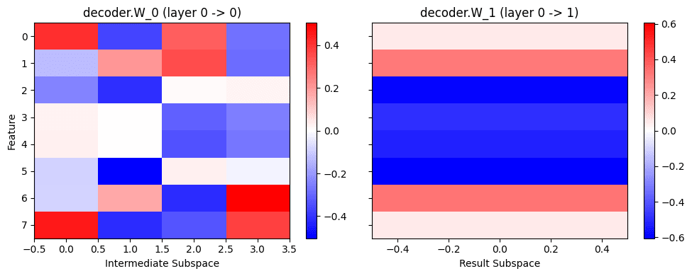
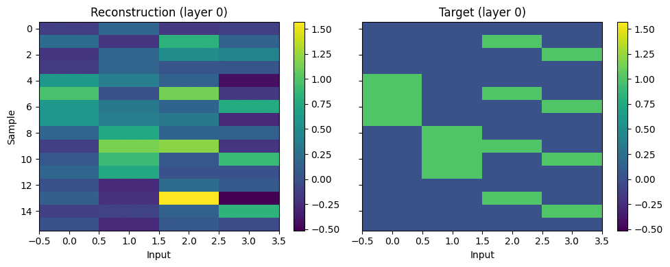
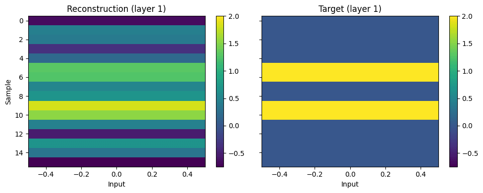
Looking at both layer-0 decoders reveals how these features in combination perfectly recover reconstructions in both layers:
To decode the final result from only layer 0 features, the decoder vector is positive for the 4 features that activate on the correct result and negative for the remainder. Because all except the correct solutions also activate on the features with negative decoder weights, they effectively cancel out.
Full Analysis of JumpReLU PLT (L0=2)
To understand what circuits the PLT learned, we plot weights, activations, and reconstructions again for the entire dataset. We show weights of alive features in both layers. Crucially, the layer-1 encoder learns non-zero weights only for the intermediate subspace efgh:
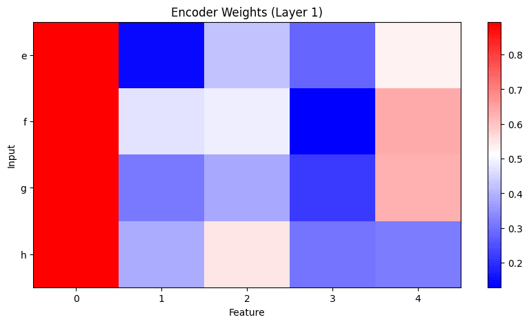
Looking at feature activations reveals that the layer-1 transcoder learned the actual behavior of layer 1: It only activates for the inputs that result in TRUE and doesn’t activate for the remaining inputs:
The decoder weights show how those features are transformed into reconstructions:
Here are the reconstructions of the PLT: