The application of residual stream sparse autoencoders (“SAEs”) to GPT-2 small reliably illustrates fundamental interpretability concepts, including feature identification, activation levels, and activation geometry.
For each category of sample text strings tested:
Both peak (single most active feature) and aggregate (total activation of the top 5 features) activation levels increased proportionally as input was progressively transformed by the model’s layers.
The most-activated feature changed for each layer, indicating a relative reshuffling of feature activity as those activity levels increase with progressive layers.
Changes in specialist scores (a measure of feature selectivity) were a mixed bag. Some categories (such as Social) activated progressively specialized features in later layers, while the remaining categories activated features with no such pattern of steadily increasing selectivity.
Confidence in these findings:
Confidence in analysis methodology: moderate-to-high
Confidence in the ability to apply these findings to more modern models: low
Introduction
The objective of this analysis is to document, in relatively simple terms, my own exploration of, and education in, concepts related to ML generally and mechanistic interpretability (“MI”) specifically, including how those concepts might be applied in practice to better understand and manage model behavior with an eye toward reducing societally harmful outputs.
This analysis does not purport to encapsulate demonstrably new findings in the field of MI. Instead, it is inspired by, and attempts to replicate at a small scale, pioneering analysis done in the field of MI by Anthropic and others, as cited below. The hope is that by replicating those analyses in plain language, from the perspective of someone with a strong interest and growing experience in MI, I might be able to add to the understanding of, discourse around, and contributions to, this field by key stakeholders who may not possess deep ML or MI expertise.
Methodology and key areas of analysis
Key areas of analysis
This analysis seeks to answer the following question: “In what ways could the use of SAEs help one understand the associative and transformative processes of a relatively simple model?”
More specifically, as a string of sample text passes through a model’s layers, how do the transformations performed on that text affect the following:
Whether the features associated with that text make intuitive “sense”: When one uses a reference such as neuronpedia.org to check the description of the features most closely associated with sample text, does that description map to the contents of that sample text? For example, are the features most activated by a string of Arabic text described as being associated with Arabic text or some other, unrelated topic?
Consistency of features most associated with the transformed text: Do the sample text’s corresponding SAE features remain the same as that text moves through the model, or do those features change as the model updates the internal representations associated with that text?
Feature activation levels and activation geometry: How do feature activation levels change as the text moves through the model’s layers? Does the feature most closely associated with that text remain equally active as the text is processed through the model? What about the top-k "constellation" of features associated with that text? How does their aggregate activation level change as the text moves through the model?
Methodology
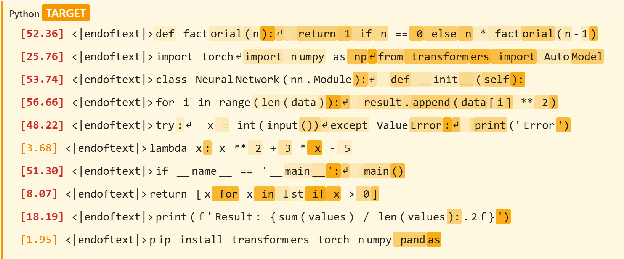
The methodology employed in my analysis was relatively straightforward. First, I used an LLM to help construct a set of sample texts designed to vary both semantically and syntactically. The logic behind this variation was to create sufficient “contrast” between the texts that would allow for easy differentiation among them by the SAE features. Those sample texts are provided in Figure 1 below.
Figure 1: Sample text used for analysis
Category
Sample Texts
Python
def factorial(n):\n return 1 if n == 0 else n * factorial(n-1)
import torch\nimport numpy as np\nfrom transformers import AutoModel
class NeuralNetwork(nn.Module):\n def __init__(self):
for i in range(len(data)):\n result.append(data[i] ** 2)
try:\n x = int(input())\nexcept ValueError:\n print('Error')
The phenomenon was observed under controlled laboratory conditions.
In accordance with the aforementioned regulations, we hereby submit this proposal.
The hypothesis was tested using a double-blind randomized controlled trial.
Pursuant to Article 12, Section 3 of the aforementioned statute.
The results indicate a statistically significant correlation (p < 0.05).
This paper examines the theoretical frameworks underlying modern economics.
The defendant pleaded not guilty to all charges in the indictment.
We acknowledge the contributions of all co-authors and funding agencies.
The experimental methodology followed established protocols.
In conclusion, further research is warranted to investigate this phenomenon.
Conver- sational
Hey, what's up? Want to grab lunch later?
I think the meeting went pretty well today.
The weather is nice, maybe we should go for a walk.
Did you see that movie everyone's talking about?
I'm planning a trip to Japan next summer.
That restaurant has the best pizza in town.
My cat keeps knocking things off the table.
The traffic was terrible this morning.
I need to finish this project by Friday.
Let's catch up over coffee sometime.
I accessed using GPT-2 Small via TransformerLens and the relevant pretrained residual stream SAEs from Joseph Bloom, Curt Tigges, Anthony Duong, and David Chanin at SAELens. I then passed each string of sample text through GPT-2 Small, using the SAEs to decompose the model's activations at layers 6, 8, 10, and 11.
In addition to recording the activation measurements provided by the relevant SAEs, I used the calculations listed below to develop a more comprehensive view of the model’s internal representation.
Specialist score
To help conceptualize and quantify the selectivity of a given SAE feature vis-a-vis the current category of sample texts, I used the following calculation:
specialist_score=ninside−noutside
wherein:
ninside = the number of text samples within a given category for which this feature has an activation level ≥ 5.0
noutside = the number of text samples outside a given category for which this feature has an activation level ≥ 5.0
It should be noted that the threshold activation level of 5.0 was chosen somewhat arbitrarily, but I do not suspect this is a significant issue, as it is applied uniformly across features and categories.
Gini coefficient:
One of the means I used to better understand the geometry of the top n most active features was via the calculation of a Gini coefficient for those features. The calculation was accomplished by sorting the activation levels and then comparing a weighted sum of activations (wherein each activation is weighted by its ranking) against its unweighted component. A Gini ranges from 0 to 1, wherein 0 indicates a perfectly equal distribution and 1 a perfectly unequal distribution (e.g. all activation resides in a single feature).
Concentration ratio (referred to as “Top5” in the table below):
To further enable an easy understanding of the top n feature geometry for a given text sample, I also calculated a simple concentration ratio that measured the total activation of the top n features for a given sample, relative to the total overall activation for that feature. While the concentration ratio thus calculated is similar to the Gini calculation described above, it tells a slightly different story. While the Gini helps one understand the geometry (i.e. the dispersion) of the top n features, relative to one another, the concentration ratio describes the prominence of those top n features relative to the overall activation associated with that sample text.
Methodological refinements
Methodological refinements made in the initial drafts of my analysis (or put more plainly, “mistakes made along the way”) were an unplanned-but-significant source of learning and are conveyed below for the benefit of the reader:
Padding masking bug: In the initial drafts of this analysis, I incorrectly included in my activation measurements, the padding used to create text samples of uniform length. Since the padding did not activate specialist features, this effectively "diluted" my results, inhibiting the emergence of the features listed in the results section below. Correcting for this issue allowed for the emergence of specialists in 5 of the 7 sample text categories in layer 6, which increased to 7 specialists by layer 11.
Mean-then-encode bug: In initial drafts of this analysis, I averaged the model activations before passing them through the SAE encoder. This essentially meant I was passing in some approximation of the sample text’s activations, not activations associated with the actual text itself. This approach was incorrect in that the SAEs were trained on actual activations, not the synthetic approximations I initially used and thus, equated to putting diesel fuel into an engine designed to burn gasoline- the input did not suit the mechanism on which it operated. Switching to an encode-then-mean approach resolved this issue and more clearly allowed for the emergence of the results shown below. Correcting for this error further improved specialist emergence, resulting in all 7 categories containing at least 1 specialist feature from layer 6 onward.
IV. Results
Summary of results
Figure 1: Summary of findings
#
Question
Findings
1
Do the features associated with that text make intuitive “sense”?
Yes: Nearly all of the most active features corresponding to each text sample are described as being thematically related to the content of that text sample.
2
Are the features most associated with the transformed text the same across layers?
No: The most activated feature for a given text sample changes by layer, shuffling among the various features associated with that concept.
3
How do feature activation levels and activation geometry vary by layer?
Activation levels: Yes Geometry: No Top feature and aggregated top-k activation levels both increase proportionally as the text moves through the model.
4
Does the selectivity of features activated by the various categories of sample text vary by category?
Yes The selectivity of the top features activated by the Social, Python, and Math categories activated more specialized features, compared to the URLs, Non-English, Formal, and Conversational categories.
Figure 2a: Summary of activation levels and geometry, by sample text category (graph)
Figure 2b: Summary of activation levels and geometry, by sample text category (table) Metrics:
Peak = single strongest feature activation
Gini = concentration of top-5 (higher = more concentrated)
Σ = sum of top-5 activations (aggregate)
Top5 = share of total activation captured by top-5 features
Spec = specialist score (strong inside − strong outside category) among the top 5 most specialized features for a given topic + layer
Click feature number to view that feature’s neuronpedia link
Finding 1: The features highlighted by the SAE make intuitive sense, relative to the associated sample text
The first area of exploration was whether the neuronpedia descriptions of the features highlighted by the SAE would have an intuitive correlation with the sample text strings that activated those features. The reader can replicate this exercise by re-running the notebook available at the project’s GitHub repository or by simply clicking the links in the table above.
While it is admittedly a qualitative assessment, the results are unambiguous: for every sample text category + layer, the most prominent feature was described on neuronpedia as being related to concepts associated with the sample text (coding conventions, html tags, etc.). In the rare instances where there was not an explicit linkage between the neuronpedia-derived description of the feature and the underlying sample text, the feature seems to have picked up on distinct syntactical elements of that sample text. For example, feature #12543 was highly activated by the Math category at layer 6 of the model. That feature is defined in neuronpedia as “special characters and symbols” and/or “caret symbols or related special characters”. While this description does not indicate math specificity, one can intuit that it was the mathematical symbology within that sample text category that likely activated this feature.
Finding 2: The top-activated feature for a given category of sample texts varies by model layer
The second area of exploration asked whether the most activated feature within a given category remained constant across layers, or if different features emerged in response to the model’s transformations. The answer seems to indicate the latter, as the most prominent feature changed at each successive model layer for each category of sample text; at no point did the same feature retain the top spot across layers.
This suggests that the transformations undertaken as inputs pass through the model not merely amplify an initial representation of that input, but rather, they materially change how those inputs are encoded.
Finding 3: Activation levels increase in later layers, but the general “shape” of that activation pattern remains relatively constant
The third avenue of my analysis asked two questions about feature behavior as input flows through successive layers of the model:
Do activation levels follow some discernible pattern?
Does the shape of that activation - the distribution of total activation - follow some discernible pattern?
With regards to the first question about activation levels, the evidence seems clear: both peak and overall activation increases as input moves through the model’s successive layers. The bars in Figure 2a clearly demonstrate this, with later activation levels being roughly 2-3x in layer 11 vs layer 6. This pattern was highly consistent in the results. Only the Social and Math categories each contained a single instance of modest peak activation decline between layers 10 and 11. The reasons for that decline, while not explored in this analysis, would be an interesting avenue for further exploration.
With regards to the second question about the shape or distribution of the feature activations observed, it seems that while peak activation levels increased in the way described above, the distribution of activations among both the top n features and the overall universe of features did not follow any significant pattern. This seems to suggest a “rising tide lifts all boats” concept in which the model’s transformations update the representation of a given input and increase the strength of that representation roughly equally across that representation’s dimensions. This is demonstrated by relatively constant Gini coefficients (indicating relatively constant distribution of activation within the top 5 features) and only modest increases in “top5” ratios (indicating relatively constant distribution of total activation between the top 5 most activated features and the thousands of less-activated features highlighted by the SAE). That this Top5 percentage hovered between roughly 3-10% for all categories and layers suggests an interesting insight: that peak activations, while useful, really only represent the “tip of the iceberg” as it relates to the model’s total internal representation. This again raises interesting prospects for further research not covered in this analysis.
Finding 4: The categories of sample text activated features of differing specificity and did so at differing layers of the model
The final avenue of exploration conducted in this analysis was an examination of the specificity of the features activated by each category, at each layer of the model. By looking at the top 5 most active features for each category + layer and then choosing the feature with the highest selectivity score (which is calculated via the methodology described above and may differ from the most active feature for that category+level), I determined the following:
Some categories, such as Social, Python, and Math developed more specialized features, compared to the remaining categories. While not proven in this analysis, one potential explanation for this behavior is that the aforementioned categories used a relatively limited and specialized set of syntax, such as emojis (Social), code snippets (Python) and mathematical operators (Math), allowing for straightforward activation of features attuned to those surface features.
Most categories showed at least some increase in feature selectivity as the input moved through the model’s layers. This again aligns with ML principles in that the transformations taking place in the model allowed for a progressively refined representation of the model inputs, which by the nature of SAE training, better corresponded with feature activation.
V. Potential avenues for further research
Examination of whether specialists are activated by syntax or semantics
One of the most interesting and unexpected observations flowing from this analysis is the apparent (but not systematically proven) activation of specialist features by the surface-level features (syntax) in the text samples, as opposed to those samples underlying meaning (semantics). Examples of this apparent phenomenon are provided in Figure 3a and Figure 3b.
While this phase of my analysis does not rigorously quantify, much less prove, the degree to which features favor syntax vs. semantics, these observations suggest a promising avenue for further research with broad implications for how we think about model control and model safety.
Exploration of the long-tail of activated features
As mentioned above, the top 5 most activated features represented only a tiny portion of the aggregate feature activation for the sample texts. This raises an obvious question as to what is going on with the remaining ~90-97% of aggregate feature activation not associated with these top 5 features. How does this “long tail” of activation change as transformations occur at each layer? What role do they play in encoding the model input? Do they associate with topic-specific features, as we saw with the most active feature for each category and layer, or do they encode some other, potentially more general concept? These are all worthwhile questions warranting further exploration.
Analysis of activation decreases
While activations increased with each progressive layer for nearly all categories, Social and Math displayed slight activation declines when comparing layer 11 to layer 10. What is the reason for this behavior? Was the occurrence of these declines at layer 11 attributable to something specific to that layer, or was that timing a simple coincidence?
Comparison with more capable models
This analysis was confined to GPT-2 Small, which is a relatively lightweight model with far more limited capabilities, compared to modern LLMs. Would the results of these analyses follow a similar pattern, if applied to a larger, more capable models, such as GPT-2 XL (1.2B parameters) or Gemma 3 via use of Google DeepMind’s Gemma Scope 2? To what degree would comparison of these analysis performed on larger models tell us about how those models’ mechanics differ and to what degree could those differences inform one’s view of the future of model development, including remaining problems to be solved?
VI. Concluding thoughts
The analysis documented here represents an honest and earnest exploration of the MI fundamentals via the use of SAEs. While the results contained within are affirmative of well-researched ML principles, replicating that research and documenting it here, proved invaluable in furthering my understanding of, and interest in, the ML principles described herein. It will no doubt serve as the springboard for my - and I hope others’ - further exploration and education into this very important topic.
I invite those interested to replicate this research using the Jupyer Notebooks available via this project’s GitHub repository and I welcome any and all comments, questions, or suggestions for improved methodologies or avenues for further research.
An exploration of SAEs applied to a small LLM
Executive summary
Findings
Confidence in these findings:
Introduction
The objective of this analysis is to document, in relatively simple terms, my own exploration of, and education in, concepts related to ML generally and mechanistic interpretability (“MI”) specifically, including how those concepts might be applied in practice to better understand and manage model behavior with an eye toward reducing societally harmful outputs.
This analysis does not purport to encapsulate demonstrably new findings in the field of MI. Instead, it is inspired by, and attempts to replicate at a small scale, pioneering analysis done in the field of MI by Anthropic and others, as cited below. The hope is that by replicating those analyses in plain language, from the perspective of someone with a strong interest and growing experience in MI, I might be able to add to the understanding of, discourse around, and contributions to, this field by key stakeholders who may not possess deep ML or MI expertise.
Methodology and key areas of analysis
Key areas of analysis
This analysis seeks to answer the following question: “In what ways could the use of SAEs help one understand the associative and transformative processes of a relatively simple model?”
More specifically, as a string of sample text passes through a model’s layers, how do the transformations performed on that text affect the following:
Methodology
The methodology employed in my analysis was relatively straightforward. First, I used an LLM to help construct a set of sample texts designed to vary both semantically and syntactically. The logic behind this variation was to create sufficient “contrast” between the texts that would allow for easy differentiation among them by the SAE features. Those sample texts are provided in Figure 1 below.
Figure 1: Sample text used for analysis
English
sational
I accessed using GPT-2 Small via TransformerLens and the relevant pretrained residual stream SAEs from Joseph Bloom, Curt Tigges, Anthony Duong, and David Chanin at SAELens. I then passed each string of sample text through GPT-2 Small, using the SAEs to decompose the model's activations at layers 6, 8, 10, and 11.
In addition to recording the activation measurements provided by the relevant SAEs, I used the calculations listed below to develop a more comprehensive view of the model’s internal representation.
Specialist score
To help conceptualize and quantify the selectivity of a given SAE feature vis-a-vis the current category of sample texts, I used the following calculation:
It should be noted that the threshold activation level of 5.0 was chosen somewhat arbitrarily, but I do not suspect this is a significant issue, as it is applied uniformly across features and categories.
Gini coefficient:
One of the means I used to better understand the geometry of the top n most active features was via the calculation of a Gini coefficient for those features. The calculation was accomplished by sorting the activation levels and then comparing a weighted sum of activations (wherein each activation is weighted by its ranking) against its unweighted component. A Gini ranges from 0 to 1, wherein 0 indicates a perfectly equal distribution and 1 a perfectly unequal distribution (e.g. all activation resides in a single feature).
Concentration ratio (referred to as “Top5” in the table below):
To further enable an easy understanding of the top n feature geometry for a given text sample, I also calculated a simple concentration ratio that measured the total activation of the top n features for a given sample, relative to the total overall activation for that feature. While the concentration ratio thus calculated is similar to the Gini calculation described above, it tells a slightly different story. While the Gini helps one understand the geometry (i.e. the dispersion) of the top n features, relative to one another, the concentration ratio describes the prominence of those top n features relative to the overall activation associated with that sample text.
Methodological refinements
Methodological refinements made in the initial drafts of my analysis (or put more plainly, “mistakes made along the way”) were an unplanned-but-significant source of learning and are conveyed below for the benefit of the reader:
IV. Results
Summary of results
Figure 1: Summary of findings
Figure 2a: Summary of activation levels and geometry, by sample text category (graph)
Figure 2b: Summary of activation levels and geometry, by sample text category (table)
Metrics:
Click feature number to view that feature’s neuronpedia link
#6501
Peak: 9.5
Gini: 0.08
Σ=39.8
Top5: 5.3%
Spec: 5
#9303
Peak: 11.5
Gini: 0.05
Σ=50.1
Top5: 5.2%
Spec: 5
#21033
Peak: 14.3
Gini: 0.02
Σ=67.4
Top5: 6.6%
Spec: 6
#8433
Peak: 21.7
Gini: 0.13
Σ=81.3
Top5: 6.9%
Spec: 6
#20051
Peak: 8.7
Gini: 0.05
Σ=36.5
Top5: 4.2%
Spec: 2
#9763
Peak: 10.9
Gini: 0.08
Σ=47.7
Top5: 4.3%
Spec: 2
#11921
Peak: 15.5
Gini: 0.07
Σ=67.5
Top5: 5.6%
Spec: 2
#16148
Peak: 18.8
Gini: 0.11
Σ=77.8
Top5: 5.5%
Spec: 2
#12543
Peak: 8.6
Gini: 0.11
Σ=33.5
Top5: 5.7%
Spec: 6
#5807
Peak: 11.8
Gini: 0.09
Σ=49.7
Top5: 6.5%
Spec: 9
#2401
Peak: 22.3
Gini: 0.13
Σ=77.5
Top5: 9.3%
Spec: 8
#24304
Peak: 19.4
Gini: 0.10
Σ=73.9
Top5: 7.4%
Spec: 6
#2351
Peak: 12.9
Gini: 0.08
Σ=54.7
Top5: 5.9%
Spec: 1
#17337
Peak: 22.6
Gini: 0.12
Σ=83.0
Top5: 6.9%
Spec: 1
#14455
Peak: 28.0
Gini: 0.08
Σ=113.8
Top5: 8.6%
Spec: 1
#9590
Peak: 37.0
Gini: 0.10
Σ=143.7
Top5: 9.9%
Spec: 2
#19212
Peak: 10.1
Gini: 0.13
Σ=37.5
Top5: 4.7%
Spec: 5
#23163
Peak: 12.0
Gini: 0.12
Σ=41.2
Top5: 4.2%
Spec: 9
#14735
Peak: 20.7
Gini: 0.18
Σ=60.6
Top5: 5.9%
Spec: 10
#9600
Peak: 18.9
Gini: 0.14
Σ=58.0
Top5: 5.0%
Spec: 10
#22570
Peak: 6.6
Gini: 0.07
Σ=27.1
Top5: 3.2%
Spec: 1
#18191
Peak: 12.3
Gini: 0.13
Σ=41.0
Top5: 3.5%
Spec: 1
#9006
Peak: 15.3
Gini: 0.09
Σ=59.9
Top5: 4.2%
Spec: 1
#19068
Peak: 25.9
Gini: 0.14
Σ=87.5
Top5: 4.9%
Spec: 2
#17244
Peak: 7.6
Gini: 0.05
Σ=32.3
Top5: 4.1%
Spec: 1
#22894
Peak: 9.7
Gini: 0.10
Σ=38.4
Top5: 3.5%
Spec: 1
#7671
Peak: 12.5
Gini: 0.09
Σ=52.7
Top5: 3.6%
Spec: 1
#23512
Peak: 14.7
Gini: 0.07
Σ=61.9
Top5: 3.3%
Spec: 2
Finding 1: The features highlighted by the SAE make intuitive sense, relative to the associated sample text
The first area of exploration was whether the neuronpedia descriptions of the features highlighted by the SAE would have an intuitive correlation with the sample text strings that activated those features. The reader can replicate this exercise by re-running the notebook available at the project’s GitHub repository or by simply clicking the links in the table above.
While it is admittedly a qualitative assessment, the results are unambiguous: for every sample text category + layer, the most prominent feature was described on neuronpedia as being related to concepts associated with the sample text (coding conventions, html tags, etc.). In the rare instances where there was not an explicit linkage between the neuronpedia-derived description of the feature and the underlying sample text, the feature seems to have picked up on distinct syntactical elements of that sample text. For example, feature #12543 was highly activated by the Math category at layer 6 of the model. That feature is defined in neuronpedia as “special characters and symbols” and/or “caret symbols or related special characters”. While this description does not indicate math specificity, one can intuit that it was the mathematical symbology within that sample text category that likely activated this feature.
Finding 2: The top-activated feature for a given category of sample texts varies by model layer
The second area of exploration asked whether the most activated feature within a given category remained constant across layers, or if different features emerged in response to the model’s transformations. The answer seems to indicate the latter, as the most prominent feature changed at each successive model layer for each category of sample text; at no point did the same feature retain the top spot across layers.
This suggests that the transformations undertaken as inputs pass through the model not merely amplify an initial representation of that input, but rather, they materially change how those inputs are encoded.
Finding 3: Activation levels increase in later layers, but the general “shape” of that activation pattern remains relatively constant
The third avenue of my analysis asked two questions about feature behavior as input flows through successive layers of the model:
With regards to the first question about activation levels, the evidence seems clear: both peak and overall activation increases as input moves through the model’s successive layers. The bars in Figure 2a clearly demonstrate this, with later activation levels being roughly 2-3x in layer 11 vs layer 6. This pattern was highly consistent in the results. Only the Social and Math categories each contained a single instance of modest peak activation decline between layers 10 and 11. The reasons for that decline, while not explored in this analysis, would be an interesting avenue for further exploration.
With regards to the second question about the shape or distribution of the feature activations observed, it seems that while peak activation levels increased in the way described above, the distribution of activations among both the top n features and the overall universe of features did not follow any significant pattern. This seems to suggest a “rising tide lifts all boats” concept in which the model’s transformations update the representation of a given input and increase the strength of that representation roughly equally across that representation’s dimensions. This is demonstrated by relatively constant Gini coefficients (indicating relatively constant distribution of activation within the top 5 features) and only modest increases in “top5” ratios (indicating relatively constant distribution of total activation between the top 5 most activated features and the thousands of less-activated features highlighted by the SAE). That this Top5 percentage hovered between roughly 3-10% for all categories and layers suggests an interesting insight: that peak activations, while useful, really only represent the “tip of the iceberg” as it relates to the model’s total internal representation. This again raises interesting prospects for further research not covered in this analysis.
Finding 4: The categories of sample text activated features of differing specificity and did so at differing layers of the model
The final avenue of exploration conducted in this analysis was an examination of the specificity of the features activated by each category, at each layer of the model. By looking at the top 5 most active features for each category + layer and then choosing the feature with the highest selectivity score (which is calculated via the methodology described above and may differ from the most active feature for that category+level), I determined the following:
V. Potential avenues for further research
Examination of whether specialists are activated by syntax or semantics
One of the most interesting and unexpected observations flowing from this analysis is the apparent (but not systematically proven) activation of specialist features by the surface-level features (syntax) in the text samples, as opposed to those samples underlying meaning (semantics). Examples of this apparent phenomenon are provided in Figure 3a and Figure 3b.
Figure 3a: Activation of “Math” feature #22917
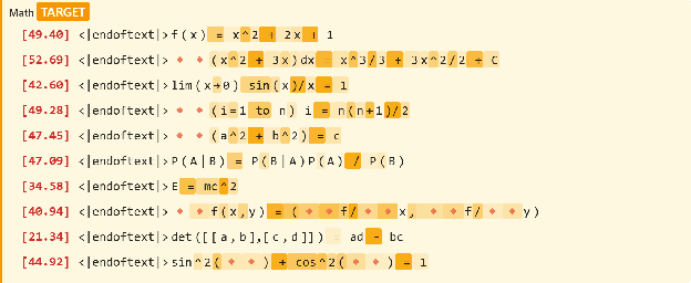
Figure 3b: Activation of “Python” feature #15983
While this phase of my analysis does not rigorously quantify, much less prove, the degree to which features favor syntax vs. semantics, these observations suggest a promising avenue for further research with broad implications for how we think about model control and model safety.
Exploration of the long-tail of activated features
As mentioned above, the top 5 most activated features represented only a tiny portion of the aggregate feature activation for the sample texts. This raises an obvious question as to what is going on with the remaining ~90-97% of aggregate feature activation not associated with these top 5 features. How does this “long tail” of activation change as transformations occur at each layer? What role do they play in encoding the model input? Do they associate with topic-specific features, as we saw with the most active feature for each category and layer, or do they encode some other, potentially more general concept? These are all worthwhile questions warranting further exploration.
Analysis of activation decreases
While activations increased with each progressive layer for nearly all categories, Social and Math displayed slight activation declines when comparing layer 11 to layer 10. What is the reason for this behavior? Was the occurrence of these declines at layer 11 attributable to something specific to that layer, or was that timing a simple coincidence?
Comparison with more capable models
This analysis was confined to GPT-2 Small, which is a relatively lightweight model with far more limited capabilities, compared to modern LLMs. Would the results of these analyses follow a similar pattern, if applied to a larger, more capable models, such as GPT-2 XL (1.2B parameters) or Gemma 3 via use of Google DeepMind’s Gemma Scope 2? To what degree would comparison of these analysis performed on larger models tell us about how those models’ mechanics differ and to what degree could those differences inform one’s view of the future of model development, including remaining problems to be solved?
VI. Concluding thoughts
The analysis documented here represents an honest and earnest exploration of the MI fundamentals via the use of SAEs. While the results contained within are affirmative of well-researched ML principles, replicating that research and documenting it here, proved invaluable in furthering my understanding of, and interest in, the ML principles described herein. It will no doubt serve as the springboard for my - and I hope others’ - further exploration and education into this very important topic.
I invite those interested to replicate this research using the Jupyer Notebooks available via this project’s GitHub repository and I welcome any and all comments, questions, or suggestions for improved methodologies or avenues for further research.