I'm very glad to see this post! Academic understanding of deep learning theory has improved quite a lot recently, and I think alignment research should be more aware of such results.
Some related results you may be interested in:
- The actual NTKs of more realistic neural networks continuously change throughout their training process, which impacts learnability / generalization
- Discrete gradient descent leads to different training dynamics from the small step size / gradient flow regime
I believe you've got a typo in the defn of
Shouldn't it be ?
Also it appears like you can simplify
Into Not sure if this wasn't done for some reason or it was a typo.
Thanks, you are right on both. I don't know how I missed the simplification, I remember wanting to make the analytical form as simple as possible.
I really should have added the reference for this, since I just copied it from a paper, so I did that in a footnote. I just followed up the derivation a bit further and the parts I checked seem solid, but annoying that it's spread out over three papers.
Nice survey, I think this line of research might be pretty important. Also worth noting that there are some significant aspects of network training that the tangent kernel model can't explain, like feature learning and transfer learning.
That makes sense to me about transfer learning, the NTK model simplifies away any path dependence during training, so we would have some difficulty using it directly as a model to understand fine-tuning and transfer learning.
But I've been a little confused about the feature learning thing since I read your post last year. I'm not sure what it means to "explain feature learning". Any Bayesian learning process is just multiplying the prior and likelihood, for each hypothesis. It seems that no feature learning is happening here? Solomonoff induction isn't doing feature learning, right?
Feature learning doesn't seem to be fundamental to interesting/useful learning algorithms, and it also seems plausible to me that a theoretical description of a learning algorithm can have no feature learning, while an efficient approximation to it with roughly the same data efficiency, could have feature learning.
Solomonoff induction isn’t doing feature learning, right?
Sure, but neural network training isn't a Bayesian black-box, it has parts we can examine. In particular we see intermediate neurons which learn to represent task-relevant features, but we do not see this in the tangent kernel limit.
it also seems plausible to me that a theoretical description of a learning algorithm can have no feature learning, while an efficient approximation to it with roughly the same data efficiency, could have feature learning
I wouldn't think of neural networks as an approximation to the NTK, rather the reverse. Feature learning makes SGD-trained neural networks more powerful than their tangent-kernel counterparts.
I don't understand why we want a theoretical explanation of neural network generalization to have the same "parts we can examine" as a neural network.
If we could describe a prior such that Bayesian updating on that prior gave the same generalization behavior as neural networks, then this would not "explain feature learning", right? But it would still be a perfectly useful theoretical account of NN generalization.
I agree that evidence seems to suggest that finite width neural networks seem to generalize a little better than infinite width NTK regression. But attributing this to feature learning doesn't follow. Couldn't neural networks just have a slightly better implicit prior, for which the NTK is just an approximation?
If we could describe a prior such that Bayesian updating on that prior gave the same generalization behavior
Sure, I just think that any such prior is likely to explicitly or implicitly explain feature learning, since feature learning is part of what makes SGD-trained networks work.
But attributing this to feature learning doesn’t follow
I think it's likely that dog-nose-detecting neurons play a part in helping to classify dogs, curve-detecting neurons play a part in classifying objects more generally, etc. This is all that is meant by 'feature learning' - intermediate neurons changing in some functionally-useful way. And feature learning is required for pre-training on a related task to be helpful, so it would be a weird coincidence if it was useless when training on a single task.
There's also a bunch of examples of interpretability work where they find intermediate neurons having changed in clearly functionally-useful ways. I haven't read it in detail but this article analyzes how a particular family of neurons comes together to implement a curve-detecting algorithm, it's clear that the intermediate neurons have to change substantially in order for this circuit to work.
Presumably the eigenfunctions are mostly sinusoidal because you're training against a sinusoid? So it's not really relevant that "it's really hard for us to express abstract concepts like 'is this network deceptive?' in the language of the kernel eigenfunctions sine wave decomposition"; presumably the eigenfunctions will be quite different for more realistic problems.
Hmm, the eigenfunctions just depend on the input training data distribution (which we call ), and in this experiment, they are distributed evenly on the interval . Given that the labels are independent of this, you'll get the same NTK eigendecomposition regardless of the target function.
I'll probably spin up some quick experiments in a multiple dimensional input space to see if it looks different, but I would be quite surprised if the eigenfunctions stopped being sinusoidal. Another thing to vary could be the distribution of input points.
Typically the property which induces sinusoidal eigenfunctions is some kind of permutation invariance - e.g. if you can rotate the system without changing the loss function, that should induce sinusoids.
The underlying reason for this:
- When two matrices commute, they share an eigenspace. In this case, the "commutation" is between the matrix whose eigenvectors we want, and the permutation.
- The eigendecomposition of a permutation matrix is, roughly speaking, a fourier transform, so its eigenvectors are sinusoids.
We don't fully understand this comment.
Our current understanding is this:
- The kernel matrix of shape takes in takes in two label vectors and outputs a real number: . The real number is roughly the negative log prior probability of that label set.
- We can make some orthogonal matrix that transforms the labels , such that the real number output doesn't change.
- This is a transformation that keeps the label prior probability the same, for any label vector.
- for all iff , which implies and share the same eigenvectors (with some additional assumption about having different eigenvalues, which we think should be true in this case).
- Therefore we can just find the eigenvectors of .
But what can be? If has multiple eigenvalues that were the same, then we could construct an R that works for all . But empirically aren't the eigenvalues of K all different?
So we are confused about that.
Also we are confused about this: "without changing the loss function". We aren't sure how the loss function comes into it.
Also this: "training against a sinusoid" seems false? Or we really don't know what this means.
Ignore the part about training against a sinusoid. That was a more specific hypothesis, the symmetry thing is more general. Also ignore the part about "not changing the loss function", since you've got the right math.
I'm a bit confused that you're calling a label vector; shouldn't it be shaped like a data pt? E.g. if I'm training an image classifier, that vector should be image-shaped. And then the typical symmetry we'd expect is that the kernel is (approximately) invariant to shifting the image left, right, up or down a pixel, and we could take any of those shifts to be R.
The eigenfunctions we are calculating are solutions to:
Where is the data distribution, is an eigenvalue and is an eigenfunction.
So the eigenfunction is a label function with input , a datapoint. The discrete approximation to it is a label vector, which I called above.
I'd expect that as long as the prior favors smoother functions, the eigenfunctions would tend to look sinusoidal?
This equation describes (almost) linear regression on a particular feature space :
This approximation isn't obvious to me. It holds if $ f(x, \theta_0) \approx 0 $ and $ \theta_0 \approx 0 $, but these aren't stated. Are they true?
Yeah good point, I should have put more detail here.
My understanding is that, for most common initialization distributions and architectures, and in the infinite width limit. This is because they both end up being expectations of random variables that are symmetrically distributed around 0.
However, in the finite width regime if we want to be precise, we can simply add those terms back onto the kernel regression.
So really, with finite width:
There are a few other very non-rigorous parts of our explanation. Another big one is that is underspecified by the data in the infinite width limit, so it could fit the data in lots of ways. Stuff about ridge regularized regression and bringing in details about gradient descent fixes this, I believe, but I'm not totally sure whether it changes anything at finite width.
From our implementation in the notebook, we can train a 3 layer ReLU network on 5 datapoints, and it tends to land on a function that looks something like this:
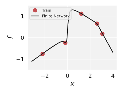
I was curious if the NTK prior would predict the two slightly odd bumps on either side of 0 on x-axis. I usually think of neural networks as doing linear interpolation when trained on tiny 1-d datasets like this, and this shape doesn't really fit that story.
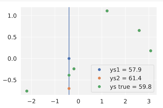
I tested this by adding three possible test datapoints and finding the log-prob of each. As you can see, the blue one has the lowest negative log-prob, so the NTK does predict that a higher data point is more likely at that location:
Unfortunately, if I push the blue test point even higher, it gets even more probable, until around y=3: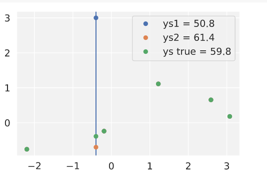
I'm confused by this. If the NTK predicts y=3 as the most likely, why doesn't the trained neural network have a big spike there?
Another test at y=0.7 to see if the other bump is predicted gives us a really weird result:
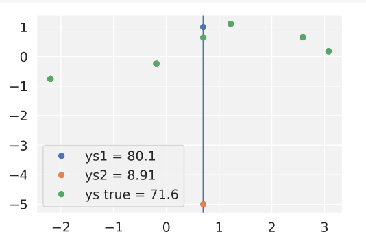
The yellow test point is by far the most a priori likely, which just seems wrong, considering the bump in the nn function is in the other direction.
Before publishing this post I'd only tested a few of these, and the results seemed to fit well with what I expected (classic). Now that I've tested more test points, I'm deeply confused by these results, and they make me think I've misunderstood something in the theory or implementation.
There was some Yannic video that I remember thinking did a good job of motivating kernels...
Aha: https://www.youtube.com/watch?v=hAooAOFRsYc
The gist being that they're nonlinearities with a "key" that lets you easily do linear operations on them.
Produced As Part Of The SERI ML Alignment Theory Scholars Program 2022 Under John Wentworth.
Introduction
Consider the following example from Goal Misgeneralization: you train an RL agent to pursue a coin, which is always at the same location (at the end of the level) during training. At test time, if the coin position is randomized, does the RL agent pursue the coin, or does it go to the fixed location?
Since the training data could not distinguish between the two goals ('go to the coin' and 'go to the location'), which one is chosen is purely based on the neural network prior. It would be nice to be able to use simplicity priors like the Solomonoff prior to think about this: the neural network might tend to choose the 'simplest' extrapolation. But what is the right notion of simplicity for neural networks? It's clearly not program length in any normal programming language, because the parity function[1] is very short but hard for neural networks to learn.
In this post, we will summarize some recent advances in DNN theory that have given us the ability to describe the prior of a deep learning network, and discuss the relevance to alignment. Our goal is to communicate quickly the insights that we found difficult to understand or slow to extract from the sources we were using.
Neural Tangent Kernel (NTK) theory compares neural networks to kernel methods. [2] The most interesting takeaways (to us) are:
Prerequisites: Linear Algebra, Gaussian Processes (GPs), to the level explained here, a source we highly recommend playing with to gain GP intuition.
Background
Notation
Let f denote the network architecture, a function that takes in the parameters and a network input, and outputs a predicted label. θ∈Rd denotes the parameters, x∈Rk is the input to the network, and y=f(θ,x)∈R is the output of the network.[3] We will use X∈Rn×k to denote the network inputs, and Y∈Rn to denote the network outputs, and denote f(θ,X) to be the network evaluated on each x in X. ϕ:Rk→Rm denotes a feature map associated with a kernel.
We will use L2 loss: L(θ)=12∑i(f(θ,xi)−yi)2.
Kernel Methods
Kernel Methods have been extensively studied in the pre-deep learning era. And it turns out that we can use insights from this area to better understand neural networks.
A kernel is a function that tells you how a priori similar any two data points are.
There are three intuitive ways I think about kernel methods:
Kernel Linear Regression
Classical linear regression works as follows: you want to find a parameter vector θ to predict data labels Y: you want Y=Xθ.[4] It's pretty easy to just solve for the θ that is closest:
Y=XθXTY=XTXθ(XTX)−1XTY=θIn order to get prediction for a new input, x, now that you have θ, you can simply multiply by theta:
^y=xθ=x(XTX)−1XTYKernel regression generalizes linear regression: instead of fitting a linear predictor from the feature space Rn, we pick a kernel function ϕ:Rn→Rm that picks out features of the input space, and then do linear regression in the higher dimensional space. We also assume that the parameters learned by the linear regression, θ, can be expressed as θ=ϕ(X)Tw, i.e., that it is a linear combination of features extracted by some feature function ϕ.[5] So:
Y=ϕ(X)θ=ϕ(X)ϕ(X)TwSolving for w gives:
w=(ϕ(X)ϕ(X)T)−1YNow, we can substitute in:
^y=ϕ(x)ϕ(X)T(ϕ(X)ϕ(X)T)−1Y=K(x,X)K−1(X,X)YThis is the equation for kernel regression, where we can understand the first two terms as being a weighted similarity vector of our test data point to each of the training data points, which is dotted with the training labels.
Neural Tangent Kernel
How are neural networks ≈ kernel methods?
Normally, you treat the neural network as f(θ,⋅), fixing θ, so you get simply a map from inputs to outputs. But there's another way of thinking about it which is as a parameter to function map, given a fixed x. In particular, we can do a Taylor expansion of the parameter function map around θ0, the initialization.
f(x,θ)≈f(x,θ0)+∇θf(x,θ0)⋅(θ−θ0)The error of this approximation is o(∥θ−θ0∥2), so the less the parameters are updated during training, the better this approximation is. One of the key results behind NTK research is that as the width of a network increases toward infinity, the parameters change less during training.
But for a moment, let's keep the width finite. At finite w, we can make a new learning algorithm called a "linearized neural network", which is described by this equation:
flinear(x,θ)=f(x,θ0)+∇θf(x,θ0)⋅(θ−θ0)This equation describes (almost) linear regression on a particular feature space ϕ(x)=∇θf(x,θ0):
flinear(x,θ)=f(x,θ0)+ϕ(x)⋅(θ−θ0)≈ϕ(x)⋅θAs we learned above in the Kernel Linear Regression section, linear regression on a feature space is equivalent to Kernel Regression with K(X,X)=ϕ(X)ϕ(X)T!
Hence, training flinear is equivalent to doing:
^y=K(x,X)K−1(X,X)Ywhere K(x1,x2)=∇θf(θ0,x1)⋅∇θf(θ0,x2).
The only major insight left is that w→∞ implies ∥θ−θ0∥→0, which means flinear→f. This is non-trivial to prove and depends on the initialization distribution.[6]
The NTK function
This Kernel regression motivates the definition of the NTK function:
NTK:Rn×Rn→Rx1,x2↦∇θf(θ,x1)⋅∇θf(θ,x2)|θ=θ0We can think of the NTK function as telling you the 'similarity' of two given data points according to the feature map at initialization. This is not to be confused with the NTK matrix: the matrix whose i,j-th component is NTK(xi,xj), for a set of input datapoints X.
The last result that we need to know is that the NTK stops depending on θ0 when the width is ∞. We won't prove this here, but the sketch is that if we expand out ∇θf(θ,x1)⋅∇θf(θ,x2)|θ=θ for a particular neural network architecture, it ends up having a lot of sums over the weights. When the width is ∞, these sums become expectations.
The NTK in the infinite width limit can be written out analytically, e.g. the one for 2 layer ReLU network is:[7]
K(x,x′)=∥x∥∥x′∥κ(x⋅x′∥x∥∥x′∥)where:
κ(u):=2u1π(π−arccos(u))+1π√1−u2Prior over data
We can view any kernel method as giving us the posterior mean of a Gaussian Process (see the Marginalization and Conditioning section of this to see why, although beware that they are using different variable names which is confusing[8]).
So we can think of the NTK as giving us a prior over the labels of a given data distribution X, specifically:
Y∼N(0,H)=e−12YTH−1Y√2πdetHWhere H is the NTK matrix, which depends on our dataset: H=∇θf(θ,X)T∇θf(θ,X). We will abbreviate the constant denominator C=√2πdetH.
Kernel Eigenmodes
We can understand this prior via eigendecomposition. Since H is positive semidefinite, it is symmetric, and so the Spectral Theorem applies, allowing us to eigendecompose H into H=PDP−1, where D is a diagonal matrix of the eigenvalues, and P is the matrix of eigenvectors of H.
Here, v1…vn are the eigenvectors of H, with corresponding eigenvalues λ1≥λ2⋯≥λn.
Eigendecomposing H gives H=PDP−1, and the labels are sampled from a Gaussian Process, so the log probability density is:
logp(Y)=log⎛⎝e−12YTH−1YC⎞⎠=−12n∑i=1(vi⋅Y)2λi−log(C)We can think of (vi⋅Y)2 as the correlation between the dataset and each eigenvector. See footnote for the full derivation.[9]
This is an explicit prior for a neural network. We can predict how a neural network will generalize to certain test points Xtest, when trained on the training data points Xtrain with labels Ytrain. The way to do this is by computing the NTK with X=[Xtest,Xtrain], then calculating logp([Ytest,Ytrain]) for several different versions of Ytest. This version of the test labels that gives the highest prior probability is the generalization most likely to be chosen. This is analogous to conditioning this Gaussian on the labels Ytrain.
Visualizing Eigenvectors
We visualize these for a specific neural network below:
When we get to the later eigenvectors, they turn out to be all sinusoidal. We can think of neural network training as finding a linear combination of these functions, where it prefers learning the functions with higher eigenvalues. It also learns the ones with higher eigenvalues earlier in training run on each of these, with update learning rate according to their eigenvalue (see appendix for why this is true).
Here is our Google Colab Notebook to generate these results.
Alignment relevance
So we have a mathematically precise notion of the simplicity prior! What does this tell us about alignment?
Unfortunately, not too much. The key problem is abstraction: it's really hard for us to express abstract concepts like 'is this network deceptive?' in the language of the kernel eigenfunctions sine wave decomposition. I am excited for future work to tackle this problem and use NTK theory to predict how neural networks will generalize. For example, could we prove something like "this neural network is very unlikely to learn an algorithm in the set of bounded tree search algorithms"?
We should be able to put any two data points into the kernel and get a measure of how similar they are. This should let us test whether the trained neural network going to treat an image of a lion in the snow as more similar to a training data point of a husky in the snow or a lion in grass?
Appendix: Modeling training dynamics with gradient flow
A result that we thought was cool that didn't fit anywhere else in this is the proof that infinitely wide neural networks can always get to zero loss. Recall that we model the training dynamics of a neural network as having infinitely small step sizes, called a gradient flow. This allows us to model training as differential equation, where we are continuously updating the parameters θ over time according to how they perform on the loss L:
˙θ(t)=−∇θL(θ(t))=−∇θ12∑i(f(θ,xi)−yi)2=−∑i∇θf(θ,xi)(f(θ,xi)−yi)=−∇θf(θ,X)⋅(f(θ,X)−Y)Where we sometimes abbreviate θ(t) as just θ. This was modeling the gradient flow in parameter space, but what we really care about is the dynamics in function space. In other words, we care about the changes in the function f(θ(t),⋅) as t increases. Fortunately, we can simply compute this on the training set:
ddtf(θ,X)=∇θf(θ(t),X)⋅˙θ(t)=−∇θf(θ,X)⋅∇θf(θ,X)⋅(f(θ,X)−Y)We have now found a crucial quantity: ∇θf(θ,X)⋅∇θf(θ,X) is the NTK matrix. Let's call it H(θ). It turns out that in the limit of width, this quantity is constant over time. Thus:
ddtf(θ,X)=−H(θ)⋅(f(θ,X)−Y)f(θ,X)=Y is clearly an equilibrium of this ODE, because when this is satisfied, the RHS is 0. We can explicitly solve this ODE by making the substitution U(t)=f(θ,X)−Y, so:
ddtU(t)=−H(θ)⋅U(t)This is a well-known ODE, with solution given by:
U(t)=e−H(θ)t⋅U(0)This gives us a proof of global convergence on the training data.
The parity function is f:{0,1}∗→{0,1}, and returns 1 if and only if the input has an odd number of ones.
See Jacot et al., Lee et al.
We will assume 1-dimensional outputs, because it makes the math much more manageable: the NTK becomes a 4-Tensor with output dimension more than 1.
Assume for simplicity that there is no noise and we can perfectly fit the data with a linear function.
There is a theorem (the Representer theorem) which says that the loss minimizing hypothesis (within the space of functions associated with this kernel) has a representation of this form.
For the actual proof, start at the bottom of p14 of the original paper and work backwards. There's a simplified version here in the One hidden Layer Network proof.
I haven't checked all of the derivation of this, I got it from On the Inductive Bias of Neural Tangent Kernels, who seem to have got it by combining the NTK definition in Appendix A of this with analytical evaluation of the integrals from here.
See the equations for conditioning a Gaussian, and assume that the prior means μX and μY are 0. Then, translating back into our variables, we get:
x|X∼N(K(x,X)K(X,X)−1Y,K(x,x)−K(x,X)K(X,X)−1K(X,x))∼N(μposterior,Σposterior)
logp(Y)=log⎛⎝e−12YTH−1YC⎞⎠=−12YTH−1Y−log(C)=−12YT(P−1DP)−1Y−log(C)=−12YTPD−1P−1Y−log(C)=−12(YTP)D−1(PTY)−log(C)=−12n∑i=1(PTY)2iλi−log(C)=−12n∑i=1(vi⋅Y)2λi−log(C)
See Jacot et al., Lee et al.