But this does not hold for tiny cosine similarities (e.g. 0.01 for , which gives a lower bound of 2 using the formula above). I'm not aware of a lower bound better than for tiny angles.
Unless I'm misunderstanding, a better lower bound for almost orthogonal vectors when cosine similarity is approximately is just , by taking an orthogonal basis for the space.
My guess for why the formula doesn't give this is because it is derived by covering a sphere with non-intersecting spherical caps, which is sufficient for almost orthogonality but not necessary. This is also why the lower bound of vectors makes sense when we require cosine similarity to be approximately , since then the only way you can fit two spherical caps onto the surface of a sphere is by dividing it into hemispheres.
This doesn't change the headline result (still exponentially much room for almost orthogonal vectors), but the actual numbers might be substantially larger thanks to almost orthogonal vectors being a weaker condition than spherical cap packing.
You made me curious, so I ran a small experiment. Using the sum of abs cos similarity as loss, initializing randomly on the unit sphere, and optimizing until convergence with LBGFS (with strong wolfe), here are the maximum cosine similarities I get (average and stds over 5 runs since there was a bit of variation between runs):
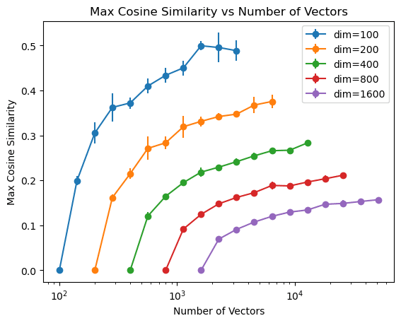
It seems consistent with the exponential trend, but it also looks like you would need dim>>1000 to have any significant boost of number of vectors you can fit with cosine similarity < 0.01, so I don't think this happens in practice.
My optimization might have failed to converge to the global optimum though, this is not a nicely convex optimization problem (but the fact that there is little variation between runs is reassuring).
I have a question about the formula. While finding the number of almost orthogonal vectors, did you use etc. to then find or was it something else?
Huge thanks for writing this! Particularly liked the SVD intuition and how it can be used to understand properties of . One small correction I think. You wrote:
is simply the projection along the vector
I think is projection along the vector , so is projection on hyperplane perpendicular to
Here are some simple Math facts rarely taught in ML & Math lectures:
SVD Is Decomposing a Matrix Into a Sum of Simple Read and Write Operations
Thanks to zfurman, on EleutherAI, which told me about the core idea.
Let's say I want to understand what a weight matrix does. A large table of numbers isn't really helpful, I want something better.
Here is a linear transformation which is much easier to understand than a table of numbers: f(x)=λ⟨v,x⟩u (where u and v are unit vectors, λ is a non-negative scalar, and ⟨v,x⟩ is the dot product between v and x). f is reading in the v direction, and writing in the u direction with a magnitude scaled by λ. I can understand this much more clearly and do nice interpretability with it. Therefore, if I know things about my embedding space (for example, using the logit lens), I can tell what f is doing.
Sadly, not all linear transformations can be expressed in this way: it's just a rank-1 transformation, so there is no hope of capturing something as complex as a usual linear transformation.
But what if I allow myself to sum many simple transformations? Then I could just look at each operation independently. More precisely, here is a wishlist to understand the big matrix M of the transformation g :
In terms of matrices, this is M=Udiag(λ)VT where U and V are semi-unitary matrices (orthogonal matrices when they are square matrices). This is exactly SVD.
Understanding matrices & SVD this way helped me find a geometric intuition behind some basic properties of matrices. The questions below can also be quickly answered by "doing the math", but I think it's interesting to have a geometric understanding of why these are true.
Feel free to share yours in the comments!
There Is Exponentially Much Room for Almost Orthogonal Vectors in High Dimensional Space
According to this paper, the number of almost orthogonal vectors you can put in n dimensional space is at least exp(nlog(1sinθ)+o(n)) where all pairs of vectors have an angle of at least θ between them (and o(n)−−−−→n→+∞0).[1]
Ignoring the o(n), and using n=1600 (the number of dimensions of the embedding space of GPT-2 XL) it means you can fit at least 3000 vectors with pairwise cosine similarities smaller than 0.1 and 1014 vectors with cosine similarities smaller than 0.2. Using n=12288 (the number of dimensions of the embedding space of GPT-3), you can fit at least 106 vectors with pairwise cosine similarities smaller than 0.05 and 10261026 vectors with cosine similarities smaller than 0.1.
This means you can get a lot of vectors in your embedding space if you allow for relatively small cosine similarities. But this does not hold for tiny cosine similarities (e.g. 0.01 for n=12288, which gives a lower bound of 2 using the formula above). I'm not aware of a lower bound better than n for tiny angles. Therefore, for a neural network to use this space to fit independent concepts, it needs to be resilient to many small-but-not-that-small conflicts.
Layer Normalization Is a Projection
Thanks to Lawrence Chan for telling me about this.
Layer Normalization is a normalization layer often found in LLMs. People usually write it as y=x−E[x]√Var[x] (followed by a scaling and a bias term[2]), which is confusing because we are taking the expected value and the variance of a vector, which is not a common geometric operation.
But it can easily be expressed in terms of two successive projection: x−E[x] is simply p→1(x), the projection on the hyperplane orthogonal to the vector →1=(1…1), p→1(x)=x−⟨x,→1⟩→1/||→1||2=x−(1d∑ixi)→1=(xj−1d∑ixi)j.
Thenx−E[x]√Var[x]=x−E[x]√E[(x−E[x])2]=p1(x)√1d∑ip1(x)2i=√dp1(x)||p1(x)||=√d pS(p1(x)), where pS is the projection on the unit sphere.
This gives us x−E[x]√Var[x]=√d pS(p1(x)).
Therefore, LayerNorm is just projecting on the hyperplane orthogonal to →1, and then projecting again on the unit sphere (of the hyperplane orthogonal to →1), times √d. These two projections are the same as projecting a point to its closest point on the unit sphere of the hyperplane orthogonal to →1[3].
For example, in dimension 3, LayerNorm is the same as projecting a point to the point of the black ring below closest to it.
This helps me see geometrically what LayerNorm(Rd) is: it's the unit sphere of the hyperplane orthogonal to 1.
This also gives me a geometrical intuition of why it might help (though the usual formula works just as well), though it is quite speculative. First, projecting on the hypersphere clearly solves the problem of exploding or vanishing activations. Second, the projection on the →1 vector pushes you away from the quadrants where ReLU is boring. Indeed, the →1 vector points towards the quadrant where all coordinates are positive, where ReLU = id, and points away from the quadrant where all coordinates are negative, where ReLU = 0. In all other quadrants, ReLU does something a bit more interesting: it zeros out some coordinates and leaves others intact.
What is missing from this geometrical point of view: It's hard to understand high dimensions. In particular, it's not easy to see that the projection on the hyperplane does almost nothing to high dimensional vectors: it only changes one coordinate among thousands. Therefore, the cosine similarity between a vector x and LayerNorm(x) is almost always very close to 1. Indeed, if ^xi are the coordinates of x in a basis which has the 1 vector (normalized) as first vector, ⟨x,LayerNorm(x)⟩||x||||LayerNorm(x)||=∑di=2^x2i√(∑di=2^x2i)(∑di=1^x2i)=√1−^x21∑di=1^x2i≈1
Appendix: Solutions to the Simple Questions Using the Geometric Interpretation of SVD
A symmetric matrix is, according to the spectral theorem, a matrix of the form Udiag(λ)UT where U is an orthogonal matrix. Therefore, a symmetric matrix is a matrix which can be decomposed as a sum of transformation of the form x↦λ⟨x,u⟩u. A symmetric matrix is the matrix of a linear transformation, which writes where it reads! Therefore, inverting a symmetric matrix is easy: if the λi are all non-zero, just read where you just wrote (in the direction of ui), scale by 1/λi, and then write back along ui. The transformation I just described to invert the action of a symmetric matrix also writes where it reads, so the inverse of a symmetric matrix is also symmetric. (You can check, that because there is no double read nor double write, what I described is legit, though the formal proof with usual linear algebra is much faster than the formal proof using geometry.)
(Udiag(λ)VT)T=Vdiag(λ)UT, therefore M transposed is the same as M, except it reads where M writes, and writes where M reads (the simple rank-1 operations are "swapped").
MMT is the composition of two linear transformations. A first one (the transposed of M, see above) which reads along ui scales by λi and writes along vi, and a second one which reads along vi, scales by λi, and writes along ui. Therefore, MMT reads along ui, scales by λ2i and writes along ui. Therefore, it is symmetric (it reads where it writes), and the ui are eigenvectors with eigenvalues λ2i because if it read ui, it will write λ2iui (there is no double read nor double writes). The same reasoning works for MTM.
Toy Models of Superposition states something similar: "It's possible to have exp(n) many "almost orthogonal" (<ϵ cosine similarity) vectors in high-dimensional spaces. See the Johnson–Lindenstrauss lemma." But this lemma does not directly state this property, and rather tells us that there is a linear map to a space with logn dimensions which almost preserves L2-distances between points. I prefer the theorem I present in this post which is directly about how many almost orthogonal vectors can fit in high-dimensional spaces.
For numerical stability reasons, people also usually add a small ϵ to the denominator.
Using the L2 distance, for a given point x, if y is the closest point to x on the unit sphere of the hyperplane H orthogonal to the 1 vector, and if pH(x) is the orthogonal projection of x on H, then by the Pythagorean theorem, d(x,y)2=d(x,pH(x))2+d(pH(x),y)2, which is minimal when y is the projection of pH(x) on the unit sphere. This proves that projecting on the unit sphere of H is the same as first projecting on H and then projecting on the unit sphere.