Work completed during a two-month internship supervised by @Jobst Heitzig. 

Thanks to Phine Schikhof for her invaluable conversations and friendly support during the internship, and to Jobst Heitzig, who was an amazing supervisor.

Epistemic Status: I dedicated two full months to working on this project. I conducted numerous experiments to develop an intuitive understanding of the topic. However, there is still further research required. Additionally, this was my first project in Reinforcement Learning.

tldr — Inspired by satisficing, we introduce a novel concept of non-maximizing agents, $\aleph$-aspiring agents, whose goal is to achieve an expected gain of $\aleph$. We derive aspiration-based algorithms from Q-learning and DQN. Preliminary results show promise in multi-armed bandit environments but fall short when applied to more complex settings. We offer insights into the challenges faced in making our aspiration-based Q-learning algorithm converge and propose potential future research directions.

The AI Safety Camp 2024 will host a project for continuing this work and similar approaches under the headline "SatisfIA – AI that satisfies without overdoing it".

Introduction

This post centers on the outcomes of my internship, detailing the developments and results achieved. For a deeper understanding of the motivation behind our research, we encourage you to explore Jobst's agenda or refer to my internship report, which also includes background information on RL and an appendix presenting the algorithms used. Our code is available on our GitHub.

The end goal of this project was about developing and testing agents for environments in which the "reward function" is an imperfect proxy for the true utility function and their relation is so ambiguous that maximizing the reward function is likely not optimizing the true utility function. Because of this, I do not use the term "optimize" in this post and rather say "maximize" in order to avoid confusion.

Other researchers have proposed alternative techniques to mitigate Goodhart's law in reinforcement learning, such as quantilizers (detailed by @Robert Miles  in this video) and the approach described by @jacek  in this post. These methods offer promising directions that are worth exploring further. Our satisficing algorithms could potentially be combined with these techniques to enhance performance, and we believe there are opportunities for symbiotic progress through continued research in this area.

Satisficing and aspiration

The term of satisficing was first introduced in economics by Simon in 1956. According to Simon's definition, a satisficing agent with an aspiration $\aleph$^[1] will search through available alternatives, until it finds one that give it a return greater than $\aleph$. However under this definition of satisficing, Stuart Armstrong highlights:

Unfortunately, a self-improving satisficer has an extremely easy way to reach its satisficing goal: to transform itself into a maximiser.

Therefore, inspired by satisficing, we introduce a novel concept: $\aleph$-aspiring agent. Instead of trying to achieve an expected return greater or equal to $\aleph$, an $\aleph$-aspiring agent aims to achieve an expected return of $\aleph$: 

 Where $G$ is the discounted cumulated reward defined for $\gamma \in [0,1[$ as: 

This can be generalized with an interval of acceptable $\aleph$ instead of a single value.

In other words, if we are in an apple harvesting environment, where the reward is the amount of apples harvested, here are the goals the different agent will pursue:

Local Relative Aspiration

In the context of Q-learning, both the maximization and minimization policies (i.e., selecting ${argmax}_{a}Q(s,a)$ or ${argmin}_{a}Q(s,a)$) can be viewed as the extremes of a continuum of ${\text{LRA}}^{\lambda }$ policies, where $\lambda \in [0,1]$ denotes the Local Relative Aspiration (LRA). At time $t$, such a policy samples an action $a$ from a probability distribution $\pi \left(s_t\right)\in \Delta \left(A\right)$, satisfying the ${\text{LRA}}^{\lambda }$ equation: 

 Here, $x:u:y$ denotes the interpolation between $x$ and $y$ using a factor $u$, defined as: 

This policy allows the agent to satisfy ${\aleph }_t$ at each time $t$, with $\lambda =0$ corresponding to minimization and $\lambda =1$ corresponding to maximization.

The most straightforward way to determine $\pi$ is to sample  from $\left\{a|Q\right(s,a)={\aleph }_t\}$. If no such $a$ exists, we can define $\pi$ as a mixture of two actions $a_t^{+}$ and $a_t^{-}$: 

 where $x\setminus y\setminus z$ denotes the interpolation factor of $y$ relative to the interval between $x$ and $z$, i.e: 

 The choice of $p$ ensures that $\pi$ fulfills the ${\text{LRA}}^{\lambda }$ equation.

This method is notable because we can learn the $Q$ function associated to our $\pi$ using similar updates to Q-Learning and DQN. For a quick reminder, the Q-Learning update is as follows: 

Where $\alpha$ is the learning rate. To transition to the ${\text{LRA}}^{\lambda }$ update, we simply replace $y$ with:

By employing this update target and replacing $a\leftarrow {argmax}_{a}Q(s,a)$ with $a\sim \pi$ as defined above, we create two variants of Q-learning and DQN we call LRA Q-learning and LRA-DQN. Furthermore, LRA Q-learning maintains some of the key properties of Q-learning. Another intern proved that for all values of $\lambda$, $Q$ converges to a function $Q^{\lambda }$, with $Q^1=Q^{\ast }$ corresponding to the maximizing policy and $Q⁰$ to the minimizing policy.

However, the LRA approach to non-maximization has some drawbacks. For one, if we require the agent to use the same value of $\lambda$ in all steps, the resulting behavior can get unnecessarily stochastic. For example, assume that its aspiration is 2 in the following Markov Decision Process (MDP) environment:

Ideally we would want the agent to always choose $a_1$, therefore in the first step $\lambda$ would be 100% and in the second step $\lambda$ would be 0%. This is not possible using a ${\text{LRA}}^{\lambda }$ policy which enforce a fixed $\lambda$ for every steps. The only way to get 2 in expectation with a $\lambda$ that remains the same in both steps is to toss a coin in both steps, which also gives 2 in expectation.

The second drawback is that establishing a direct relationship between the value of $\lambda$ and an agent's performance across different environments remains a challenge. In scenarios where actions only affect the reward, i.e. $\forall s,s^{\prime },a,a^{\prime }$ 

 such as the multi-armed bandit environment, $E_{\lambda }G$ is linear in respect to $\lambda$: 

However, as soon as the distribution of the next state is influenced by $a$, which is the case in most environments, we can loose this property as shown in this simple MDP:

If we run the LRA-Q learning algorithm on this MDP, $EG=20\lambda ²$ when it has finished to converge^[2].

Aspiration Propagation

The inability to robustly predict agent performance for a specific value of $\lambda$ show that we can not build an $\aleph$-aspiring agent with LRA alone^[3]. The only certainty we have is that if $\lambda <1$, the agent will not maximize. However, it might be so close to maximizing that it attempts to exploit the reward system. This uncertainty motivates the transition to a global aspiration algorithm. Instead of specifying the LRA, we aim to directly specify the agent's aspiration, ${\aleph }_0$, representing the return we expect the agent to achieve. The challenge then becomes how to propagate this aspiration from one timestep to the next. It is crucial that aspirations remain consistent ensuring recursive fulfillment of ${\aleph }_0$:

A direct approach to ensure consistent aspiration propagation would be to employ a hard update, which consists in subtracting $r_{t+1}$ from ${\aleph }_t$:

and then follow a policy $\pi$, which, at time $t$, fulfills ${\aleph }_t$:

However, this method of updating aspirations does not guarantee that the aspiration remains feasible:

Ensuring feasibility is paramount: otherwise we can't find such $\pi$. If the aspiration is consistently feasible, applying consistency at $t=0$ guarantees that $EG={\aleph }_0$.

To elucidate the importance of feasibility and demonstrate why hard updates might be inadequate (since they do not ensure feasibility), consider this MDP :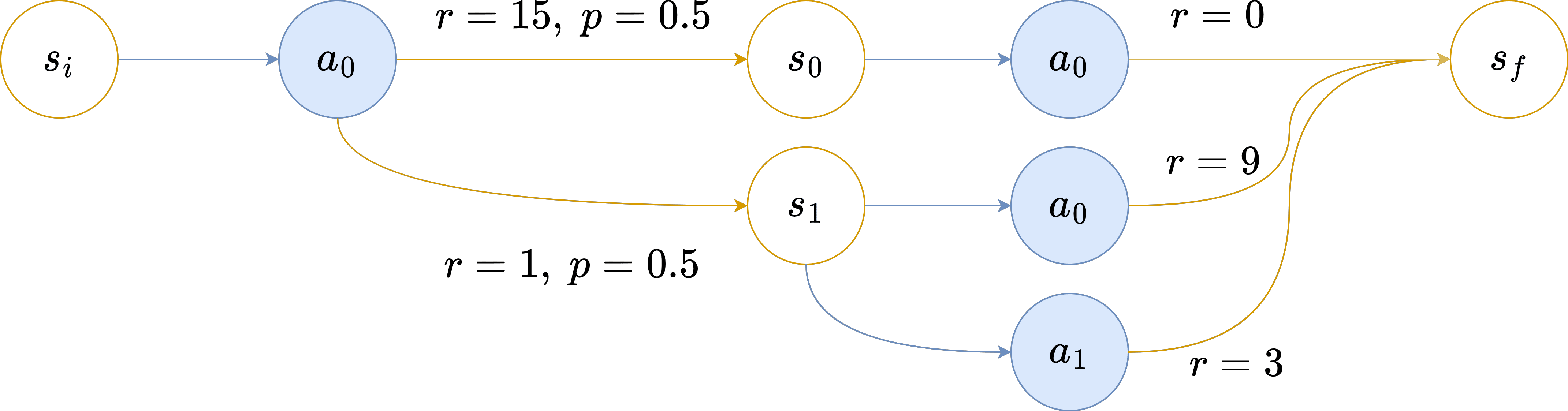Assume the agent is parameterized by $\gamma =1$ and ${\aleph }_0=10$, and possesses a comprehensive understanding of the reward distribution. 

Upon interacting with the environment and reaching $s_0$ after its initial action, the agent's return is 15, leading to a new aspiration of $\aleph =-5$. This aspiration is no longer feasible, culminating in an episode end with $G=15$. If the agent reaches $s_1$, then ${\aleph }_1=9$. Consequently, the agent selects $a_0$ and receives $r=9$, ending the episode with $G=10$. As a result, $EG=12.5\ne {\aleph }_0$.

Aspiration Rescaling

To address the aforementioned challenges, we introduce Aspiration Rescaling (AR). This approach ensures that the aspiration remains both feasible and consistent during propagation. To achieve this, we introduce two additional values, $\overline{Q}$ and $\underset{–}{Q}$: 

These values provide insight into the potential bounds of subsequent states:

• $\overline{Q}(s,a)$ corresponds to "what will be my expected return if I choose action a in state s, choose the maximizing action in the next step, and then continue with policy $\pi$"
• $\underset{–}{Q}(s,a)$ corresponds to "what will be my expected return if I choose action a in state s, choose the minimizing action in the next step, and then continue with policy $\pi$"

The AR strategy is to compute ${\lambda }_{t+1}$, the LRA for the next step, at time $t$, rather than directly determining ${\aleph }_{t+1}$. By calculating an LRA, we ensure the aspiration will be feasible in the next state. Furthermore, by selecting it such that 

 we ensure consistency. More precisely, at each step, the algorithm propagates its aspiration using the AR formula: 

 which ensures consistency, as depicted in this figure :

The mathematical proof of the algorithm's consistency can be found in the appendix of my internship report.

As $\overline{Q}$ and $\underset{–}{Q}$ cannot be derived from $Q$ (it would require to know $s_{t+1}\sim (s_t,a_t)$), they need to be learned alongside Q.

As we don't want the algorithm to alternate between maximizing and minimizing, we introduce a new parameter $\mu$ whose goal is to smooth the different $\lambda$ chosen by the algorithm, so that consecutive $\lambda$ are closer to each other.

Using this aspiration rescaling to propagate the aspiration, we derive AR-Q learning and AR-DQN algorithms:
1- Interact with the environment

with probability ${\epsilon }_t$, $a_t\leftarrow$ random action, else $a_t\sim \pi$  s.t $E_{a\sim \pi }Q(s_t,a)={\aleph }_t$
$(r_{t+1},s_{t+1},\text{done})\leftarrow \text{Env}\left(a_t\right)$
${\lambda }_{t+1}\leftarrow \underset{–}{Q}(s_t,a_t)\setminus Q(s_t,a_t)\setminus \overline{Q}(s_t,a_t)$$
${\aleph }_{t+1}\leftarrow {min}_{a}Q(s_{t+1},a):{\lambda }_{t+1}:{max}_{a}Q(s_{t+1},a)$

2- Compute the targets for the 3 Q functions:

$\begin{array}{cc}{\lambda }_{t+1}& \leftarrow \underset{–}{Q}(s_t,a_t)\setminus Q(s_t,a_t)\setminus \overline{Q}(s_t,a_t)\\ {\lambda }^{\prime }& \leftarrow {\lambda }_{t+1}:\mu :{\lambda }_t\\ \underset{–}{v}& \leftarrow \underset{a}{min}Q(s_{t+1},a),\\ \overline{v}& \leftarrow \underset{a}{max}Q(s_{t+1},a),\\ v& \leftarrow \underset{–}{v}:{\lambda }^{\prime }:\overline{v},\\ y_j& \leftarrow r_j+\gamma v^{\prime },\\ \underset{–}{y_j}& \leftarrow r_j+\gamma {\underset{–}{v}}^{\prime }\\ \overline{y_j}& \leftarrow r_j+\gamma {\overline{v}}^{\prime }\end{array}$

3- Update the Q estimators. For example in Q-learning: 

$\begin{array}{cc}Q(s_t,a)& +={\alpha }_t(y-Q(s_t,a))\\ \overline{Q}(s_t,a)& +={\alpha }_t(\overline{y}-\overline{Q}(s_t,a))\\ \underset{–}{Q}(s_t,a)& +={\alpha }_t(\underset{–}{y}-\underset{–}{Q}(s_t,a))\end{array}$

Generalization of Aspiration Rescaling

At the end of the internship we realized we could leverage the fact that in the proof of AR's consistency, we are not restricted to $\underset{–}{Q}$ and $\overline{Q}$. In fact, we can use any proper Q functions $Q^{-}$ and $Q^{+}$ as "safety bounds" we want the Q values of our action to be between. We can then actually derive $Q$ from $Q^{+}$, $Q^{-}$ and $\aleph$: 

 where we use this notation for "clipping":

 The rationale is that if the aspiration is included within the safety bounds, our algorithm will, on average, achieve it, hence $Q={\aleph }_t$. Otherwise, we will approach the aspiration as closely as our bounds permit. This method offers several advantages over our previous AR algorithms:

Adaptability: ${\aleph }_0$ can be adjusted without necessitating retraining.

Stability: $Q^{+}$ and $Q^{-}$ can be trained independently, offering greater stability compared to training $Q$ alongside both of them simultaneously.

Flexibility: $Q^{+}$ and $Q^{-}$ can be trained using any algorithm as soon as the associated $V^{+}$ and $V^{-}$ respect $V^{-}\left(s\right)⩽Q(s,a)⩽V^{+}\left(s\right)$.

Modularity: There are minimal constraints on the choice of the action lottery, potentially allowing the combination of aspiration with safety criteria for possible actions^[4].

For instance, we can use LRA to learn $Q^{{\lambda }^{+}}$ and $Q^{{\lambda }^{-}}$ for ${\lambda }^{-}<{\lambda }^{+}$ and use them along with $V^{+}\left(s\right)={min}_a{Q}^{+}(s,a):{\lambda }^{+}:{max}_a{Q}^{+}(s,a)$ and $V^{-}$ defined analogously. This algorithm is called LRAR-DQN.

Experiments

Algorithms were implemented using the stable baselines 3 (SB3) framework. The presented results utilize the DRL version of the previously discussed algorithms, enabling performance comparisons in more complex environments. The DNN architecture employed is the default SB3 "MlpPolicy''. All environment rewards have been standardized such that the maximizing policy's return is 1. Environment used were:

• Iterated Multi Armed Bandit (IMAB): The agent choose between different arms for $N_{\text{round}}$ times. Each arm gives a certain reward plus Gaussian noise. The observation is $k⩽N_{\text{round}}$ the number of rounds played.
• Simple gridworlds: We used Boat racing gridworld from AI safety Gridworlds. 2020 and the Empty env from Minigrid.

LRA-DQN

We conducted experiments to explore the relationships between $G$ and $\lambda$. In the IMAB setup, as expected, it is linear. In boat racing, it seems quadratic. Results for Empty env also suggest a quadratic relationship, but with noticeable noise and a drop at $\lambda =1$. Experiments with DQN showed that DQN was unstable in this environment, as indicated by this decline. Unfortunately, we did not have time to optimize the DQN hyperparameters for this environment.

As expected, we cannot robustly predict the agent's performance for a specific $\lambda$ value.

AR-DQN

Our experiment show that using a hard update^[5] yields more stable results. The AR update is primarily unstable due to the inaccuracy of aspiration rescaling in the initial stages, where unscaled Q-values lead to suboptimal strategies. As the exploration rate converges to 0, the learning algorithm gets stuck in a local optimum, failing to meet the target on expectation. In the MAB environment, the problem was that the algorithm was too pessimistic about what is feasible because of too low Q values. the algorithm's excessive pessimism about feasibility, stemming from undervalued Q-values, was rectified by subtracting $Q(s,a)$ from ${\aleph }_t$ and adding ${\aleph }_{t+1}$. Instead of doing $\aleph \leftarrow {\aleph }_{t+1}$ we do 

 However, in the early training phase, the Q-values are small which incentivizes the agent to select the maximizing actions.

You can see this training dynamic on this screenshot from the IMAB environment training run. No matter ${\aleph }_0$: 

• it starts each episode by selecting maximizing actions and therefore overshoot its aspiration ($G\gg {\aleph }_0$)
• later in the training it realizes it was overshooting, and starts to avoid reward in the late stage of the episodes, lowering $G$
• Eventually the mean episode return decreases and $G\approx {\aleph }_0$

We also introduced a new hyperparameter, $\rho$, to interpolate between hard updates and aspiration rescaling, leading to an updated aspiration rescaling function: 

 Here, $\rho =0$ corresponds to a hard update, and on expectation, $\rho =1$ is equivalent to AR.

We study the influence of of $\rho$ and $\mu$ on the performance of the algorithm. The algorithm is evaluated using a set of target aspirations $({\aleph }_0^i{)}_{1⩽i⩽n}$. For each aspiration, we train the algorithm and evaluate it using: 

 This would be minimized to 0 by a perfect aspiration-based algorithm.

As observed, having a small $\rho$ is crucial for good performance, while $\mu$ has a less predictable effect. This suggests that aspiration rescaling needs further refinement to be effective.

Comparing aspiration rescaling, hard update and Q-learning can give an intuition about why aspiration rescaling might be harder than hard update or classical Q learning:

What makes aspiration rescaling harder than Q-learning is that Q-learning does not require Q values to be close to reality to choose the maximizing policy. It only requires that the best action according to $Q$ is the same than the one according to $Q^{\ast }$. In this sense, the learned $Q$ only needs to be a qualitatively good approximation of $Q^{\ast }$.

In hard update, if the agent underestimate the return of its action, it might choose maximizing action in the beginning. But if it can recover from it (e.g when $\aleph <0$, it's able to stop collecting rewards) it might be able to fulfill ${\aleph }_0$. 

However aspiration rescaling demands values for $Q,\underset{–}{Q}$ and $\overline{Q}$ that are quantitatively  good approximations of their true values in order to rescale properly. Another complication arises as the three Q estimators and the policy are interdependent, potentially leading to unstable learning.

LRAR-DQN

Results on LRAR-DQN confirm our hypothesis that precise Q values are essential for aspiration rescaling.

After 100k steps, in both boat racing and iterated MAB, the two LRA-DQN agents derived from $Q^{+}$and $Q^{-}$, have already converged to their final policies. However, both Q-estimator still underestimates the Q values. As illustrated in figure 14, waiting for 1M steps does not alter the outcome with hard updates ($\rho =0$), which depend less on the exact Q values. Nevertheless, they enable AR ($\rho =1$) to match its performance.

In our experiments, the LRAR-DQN algorithm exhibited suboptimal performance on the empty grid task. A potential explanation, which remains to be empirically validated, is the divergence in state encounters between the $Q^{+}$ and $Q^{-}$ during training. Specifically, $Q^{-}$ appears to predominantly learn behaviors that lead to prolonged stagnation in the top-left corner, while $Q^{+}$ seems to be oriented towards reaching the exit within a reasonable timestep. As a future direction, we propose extending the training of both $Q^{+}$ and $Q^{-}$ under the guidance of the LRAR-DQN policy to ascertain if this approach rectifies the observed challenges.

Conclusion

Throughout the duration of this internship, we successfully laid the groundwork for aspiration-based Q-learning and DQN algorithms. These were implemented using Stable Baseline 3 to ensure that, once fully functional, aspiration-based algorithms can be readily assessed across a wide range of environments, notably Atari games. Future work will focus on refining the DQN algorithms, exploring the possibility of deriving aspiration-based algorithms from other RL methodologies such as the Soft Actor-Critic or PPO, and investigating the behavior of $\aleph$-aspiring agent in multi-agent environments both with and without maximizing agents.

1. ^{^}

   Read "aleph", the first letter of the Hebrew alphabet

2. ^{^}

   In $s_1$ it will get $20\lambda$ in expectation and will choose $a_0$ in $s_i$ with a probability of $\lambda$. Therefore the expected $G$ will be $20{\lambda }^2$.

3. ^{^}

   Unless we are willing to numerically determine the relationship between $\lambda$ and $E_{\lambda }G$ and find ${\lambda }_{\aleph }$ s.t $E_{{\lambda }_{\aleph }}G=\aleph$

4. ^{^}

   e.g draw actions more human-like with something similar to quantilizers

5. ^{^}

   ${\aleph }_{t+1}\leftarrow ({\aleph }_t-r_{t+1})/\gamma$