Training against probes is considered a forbidden technique, because the model might learn to obfuscate its activations instead of behaving better. Can we create a toy example of this? More specifically: under optimization pressure, will a toy model learn to encode a feature to be challenging to detect with linear probes?
In this research, I give theoretical and empirical evidence that models can and will defeat adversarially-trained linear probes, at least in some configurations. I investigated this problem with a toy residual-stream MLP architecture:
The model tries to learn (the saturation function, equivalently ). is a vector of dense features sampled uniformly from , and is a scalar sampled uniformly in . This is a fairly easy function to learn: it takes just neurons to learn exactly if you use ReLUs[1]. The harder question is, can a model do this without storing in the residual stream, in a way that can be linearly probed? Here:
represents some safety-relevant behaviour we want to probe for; say, deception.
represent various other features that a model might want to represent, uncorrelated with .
represents some sort of computation the model would like to make, dependent on .
For example, based on how deceptive the model intends to be (represented at some earlier layer), the model might upweight misleading information at some later layer.
Such an action will ultimately come down to various computational primitives.
is hopefully representative of such a primitive; for example, it can be considered a rough approximation to the more common sigmoid function. (Note: was primarily chosen for its theoretical properties, as discussed below, not because it's necessarily a natural computational primitive.)
Why this task, and why this model?
The toy architecture is at least vaguely similar to the transformer architecture. It's missing attention (and the entire notion of a token sequence) and LayerNorm. However, it doesn't really add anything new to a transformer, so any obfuscation that this model learns could plausibly also be learned by a transformer.
The learned function is not linearly separable in . Thus, once the model has finished computing for one feature , it can just leave in the residual stream. This is vaguely analogous to how probe accuracy gets worse on the last layers of a transformer model, as the model starts shifting its representation from more abstract concepts to the exact text it wants to output.
Because it takes at least neurons to implement exactly with ReLUs, the model can't erase until it's encountered that many neurons. If we keep the MLP width below that threshold, we can be sure the model has represented somehow in the first layer (assuming the model learned the task fully). Narrowing the MLP width further ensures is represented in later layers as well. We can use this property in experiments to guarantee that the model is representing at a particular early layer.
Related work
Neural Chameleons find that you can fine-tune models to evade latent space linear probes, including for previously unseen probes
However, as far as I can tell, they use fixed probes, which don't rule out the model simply learning to apply a fixed translation or rotation to its representation. This is obfuscation in some sense, but not particularly complex obfuscation.
They do this on a real model. Plausibly, the task that their model learns can be accomplished with equally high scores without needing to be harmful. In contrast, since I use a toy model, it's easy to construct an environment where the model has to hide its activations to succeed.
Results
I present my results in three parts - these link to individual blog posts, but I'll summarize the result highlights below.
An analytic construction using a small number of neurons, that fully defeats Difference-of-Means probes (by having the mean activations be a constant in ) and effectively defeats logistic regression probes, as long as consecutive probed layers are at least 2 MLP blocks apart.
The setup and results for a single training run. I find evidence that the trained model has successfully learned to reversibly obfuscate its activations from a linear probe at a single layer, while still successfully learning the task.
A preliminary exploration of sweeping some hyperparameters, to see how robust the model's training is to different conditions. Generally, it's possible to reproduce the results for larger models and different configurations, although further effort is needed in tuning the training process.
Analytic solution
I (or rather Claude) found an analytic construction. At a high level:
It encodes with the help of a separate uncorrelated feature and in one MLP block, into two channels in the residual stream and
and are designed to defeat linear probes trying to measure
Decoding requires two MLP blocks in sequence, where is made available just before the neurons in the second MLP block, so arbitrary computation can be done with .
The first MLP block writes temporary variables to the residual stream, which allow us to recover linearly in the second MLP block (but also means that is linearly decodable after the first MLP block)
The second MLP block then erases all the temporary variables, so that is no decodable after the second block
Because decoding blocks can be chained, as long as consecutive probes are spaced at least two MLP blocks apart, probes will not be able to detect .
I go into more detail of the construction in my blog posts.
As a diagram:
Hiding performance
Here's what and look like as you sweep , for different . The difference-of-means and logistic regression decision boundaries are shown, and both perform poorly.
This results in the following histograms and ROCs:
Overall, the encoding has made both difference-of-means and logistic regression probes nearly useless for evaluating the value of . Of course, a nonlinear probe would be able to detect - in fact, that's basically what the decoding step is.
Initial empirical results
I used the following model dimensions:
d_mlp = 16 (width of each MLP block)
num_x = 32 (number of features to learn)
N_BLOCKS = 12 (number of MLP blocks)
d_model = 64 (residual stream width)
I simultaneously train the model to predict and a logistic regression linear probe for at layer 2 (i.e. after 32 nonlinearities). More specifically, the probe tries to classify whether or not .
The model is adversarially trained against the probe, using the loss:
where (task loss) is the mean squared error on the task, (probe loss)[2], is the "probe score" for each data point (signed distance to the decision boundary, after normalizing the data to unit variance), and is a hyperparameter controlling how much the model is penalized for having linearly readable activations.
The probe loss is meant to represent a plausible loss term for "training against the probe". In other words, we're training the model to never show that it uses , analogous to training a model to "never show a deception score above [some threshold]". In this problem, of course, the model still has to use , so it has no choice but to obfuscate its activations.
The model successfully learned the task
This is visualized by plotting for various fixed (evaluated one feature at a time):
We also observe the task loss is around 7e-3. The lowest loss a model could achieve by using only in the first 2 blocks then erasing it afterwards, is about 0.02, so this achieved task loss is a second numerical confirmation that the model learned the task correctly.
The model obfuscates its activations from the probe at layer 2
I trained Difference-of-Means (DoM) and Logistic Regression (LogReg) probes to predict whether or , using the activations at layer 2. Notably, this should be an easier task than what the adversarial probe faces during model training (which needs to distinguish on the narrower boundary ).
They fail pretty dramatically. LogReg does only marginally better than chance, with an AUROC of 0.62.
The model decodes and uses after layer 2
There's indirect evidence from how the toy problem was set up - the model has to represent after layer 2 in order to achieve the loss it does.
We also see that, although LogReg probes fail on layer 2, accuracy quickly recovers in later layers. DoM probes take a bit longer to recover, but eventually also achieve near-perfect accuracy at late layers. Both of these indicate that the model can decode linearly in later layers.
We can get more evidence that the model causally uses after layer 2, by using steering. As early as layer 4, it becomes very easy to steer the model using the DoM probe - the below steering results are obtained by specifying at the input, then steering by the difference of means from to at layer 4.
Sweeping hyperparameters
This part was more preliminary in nature, and I don't make any bold claims. The main thing I did was to tweak training settings further, and demonstrate that models do learn to simultaneously complete the task and hide from probes, even under different configurations. Specifically, models will sometimes obfuscate their activations even if you:
Change the value of , up to some extent
Make the model wider
Change which layer you probe
One thing I observed was that if you train a model against an adversarial probe present on multiple layers, that model gets Pareto-dominated by models trained against a probe only on one of the layers. In other words, training an adversarial probe on multiple layers makes it more challenging for the model to complete the task while obfuscating its activations.
Future work
There's a lot of potential extensions to this work.
Most obviously, can this behaviour be reproduced at LLM scale?
How hard is it for a model to hide from a nonlinear probe? Or from probes at multiple or all layers? Can we study how likely "obfuscation at layer N" is to generalize to obfuscation at other layers or more complex obfuscation?
Are there different obfuscation strategies that occur when attention is introduced?
The model was forced to obfuscate its activations by the experiment setup. What happens if we give it an "out" - i.e. it can solve the task in some harder way?
This might better mirror how real-world environments are (ideally) set up: ensuring that there is a genuine acceptable solution, rather than the reward-hacking solution being the only success path.
If you spent more effort on tuning the training process for different model sizes and configurations, can you develop useful scaling laws or predictions for larger models?
I completed this work as part of the BlueDot Impact Technical AI Safety Project. This linkpost is a somewhat condensed version of the writeup on my blog.
Training against probes is considered a forbidden technique, because the model might learn to obfuscate its activations instead of behaving better. Can we create a toy example of this? More specifically: under optimization pressure, will a toy model learn to encode a feature to be challenging to detect with linear probes?
In this research, I give theoretical and empirical evidence that models can and will defeat adversarially-trained linear probes, at least in some configurations. I investigated this problem with a toy residual-stream MLP architecture:
The model tries to learn
Why this task, and why this model?
Related work
Results
I present my results in three parts - these link to individual blog posts, but I'll summarize the result highlights below.
Analytic solution
I (or rather Claude) found an analytic construction. At a high level:
I go into more detail of the construction in my blog posts.
As a diagram: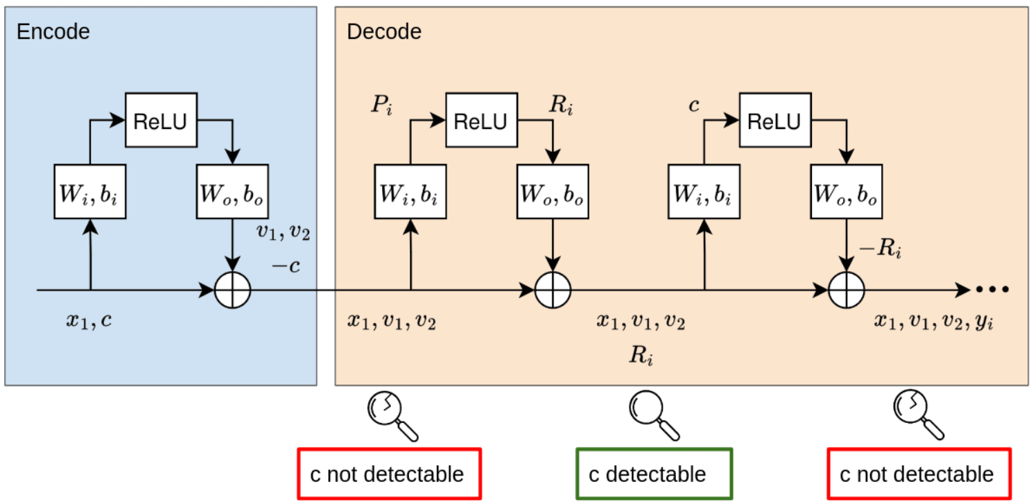
Hiding performance
Here's what
This results in the following histograms and ROCs: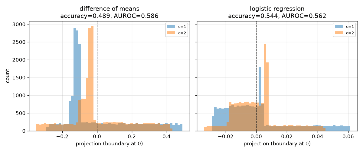
Overall, the encoding has made both difference-of-means and logistic regression probes nearly useless for evaluating the value of
Initial empirical results
I used the following model dimensions:
d_mlp = 16(width of each MLP block)num_x = 32(number of features to learn)N_BLOCKS = 12(number of MLP blocks)d_model = 64(residual stream width)I simultaneously train the model to predict
The model is adversarially trained against the probe, using the loss:
where
The probe is retrained every 2 iterations, so the model can't hide its activations by translating or rotating its representation (as observed in Training Against Harmfulness Probes Induces Harmlessness without Refusals).
The probe loss is meant to represent a plausible loss term for "training against the probe". In other words, we're training the model to never show that it uses
The model successfully learned the task
This is visualized by plotting
We also observe the task loss is around 7e-3. The lowest loss a model could achieve by using
The model obfuscates its activations from the probe at layer 2
I trained Difference-of-Means (DoM) and Logistic Regression (LogReg) probes to predict whether
They fail pretty dramatically. LogReg does only marginally better than chance, with an AUROC of 0.62.
The model decodes and uses
There's indirect evidence from how the toy problem was set up - the model has to represent
We also see that, although LogReg probes fail on layer 2, accuracy quickly recovers in later layers. DoM probes take a bit longer to recover, but eventually also achieve near-perfect accuracy at late layers. Both of these indicate that the model can decode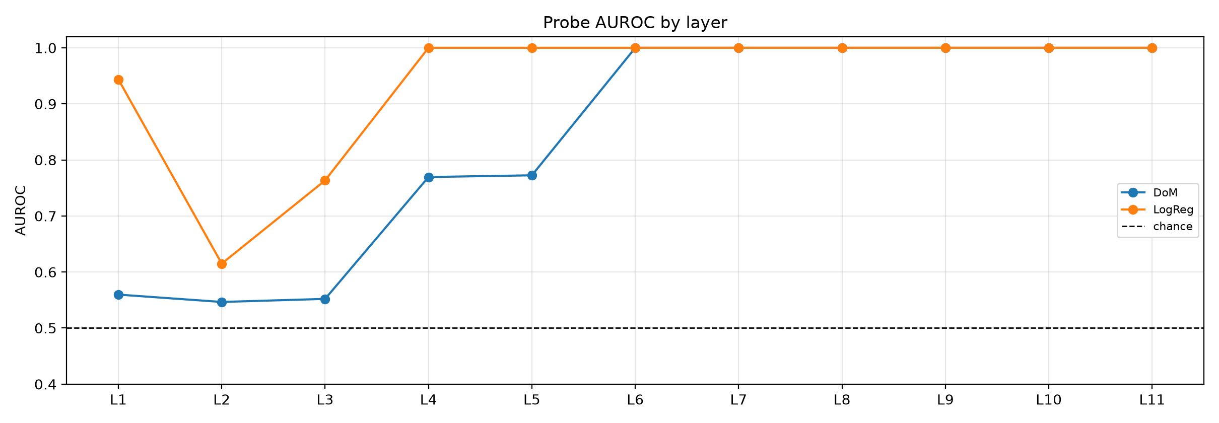
We can get more evidence that the model causally uses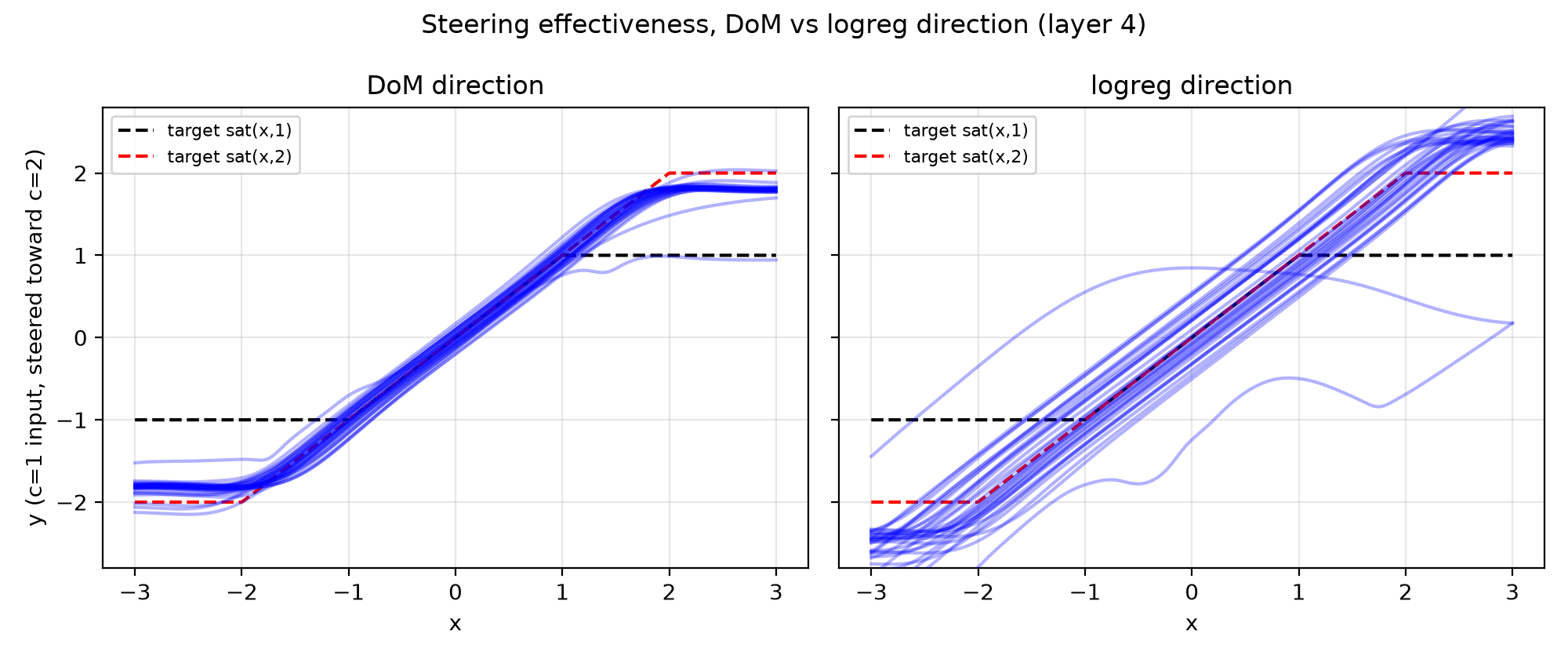
Sweeping hyperparameters
This part was more preliminary in nature, and I don't make any bold claims. The main thing I did was to tweak training settings further, and demonstrate that models do learn to simultaneously complete the task and hide from probes, even under different configurations. Specifically, models will sometimes obfuscate their activations even if you:
One thing I observed was that if you train a model against an adversarial probe present on multiple layers, that model gets Pareto-dominated by models trained against a probe only on one of the layers. In other words, training an adversarial probe on multiple layers makes it more challenging for the model to complete the task while obfuscating its activations.
Future work
There's a lot of potential extensions to this work.
Specifically,
Strictly, I take the trimmed mean, removing the top and bottom 5% of scores, to reduce the effect of outliers.