The second way gradient descent is used is to find the activations of the neural network, in this case, to find the values of the , given a single input image. This is not standard from the perspective of modern deep learning, but should set off mesa-optimizer alarm bells.
Actually this is completely standard in DL as it's core functionality of the transformer architecture. Transformers consist of a stack of homogeneous layers that update a shared residual stream, so they are residual networks and thus equivalent to an unrolled iterative estimator with untied weights. In this form it's more obvious that transformers are equivalent to (constrained) unrolled recurrent networks that performs K iterative sub inference steps on a probability map (the residual stream) per main token prediction step.
In this sense they are much closer to brain arch than most realize. Each main 'layer' (or sub step in the shared weight form) has two sub modules: a pure depth 2 FF network which is a close match for the cerebellum in the brain, and the attention submodule which provides short term contextual memory - and is thus arguably more similar to the recurrent modules of the cortex/hippocampus (due to the equivalence of fast weight RNNs and transformer attention modules).
So if you imagine implementing a large transformer physically with a huge but slow circuit, each main layer (with its own weights) would correspond to a cortical-cerebellar module pair, with the cortical module as the attention part and the cerebellar module as the FF part. Full pipeline parallelization is used of course, so that temporal flow down the transformer depth corresponds to flow from sensory up to higher level modules and then down to motor modules in the brain.
There are some differences of course - the brain arch is truly recurrent, which would be like allowing connections from higher levels down to lower levels in the transformer depth. Transformers dont allow this because it breaks their parallelization over time strategy, which is their major serious weakness compared to the more fully universal RNN arch of the brain.
There are many many other convergent details of course - the bits per weight of the most efficient transformers is converging to 4-bits per weight similar to the brain, the #weights per neuron is similar, the learned internal representations are similarish or functionally equivalent, etc
Why is it called predictive "coding" in the first place? Also this particular method didn't end up as being very useful compared to neural networks, right? So what is the relevance of it?
It’s called predictive coding because you’re encoding the image as the vector r, which is typically much smaller than the image. The idea is that in the brain, U changes slowly, while r tracks changes in the retinal image.
It’s not the best method for machine learning, but some smart people claim this is our best bet for the algorithm actually used by the brain. So it is of interest for that reason alone. In addition, there’s a good chance that our current algorithms are not the best possible, so it behooves us to keep some “also ran” algorithms in mind. It’s happened several times in the history of AI that an apparently inferior algorithm has received a minor tweak and become a champion.
Just to add to Carl Feynman's response, which I thought was good.
Part of the reason these systems are inefficient is because it requires you to (effectively) run gradient descent even at inference, even after training is over. Or you can run the RNN, which is mathematically equivalent but again you can see where the inefficiency comes in: the value at time t=3 is a function of the value at time t=2, which is a function of t=1 and so on, so in order to get the converged value of the activations you have to, in a for loop, compute each timestep one by one.
This is in contrast to a feedforward network like a (normal) convnet or transformer, which can run extremely quickly and in parallel on gpu.
Great explanation, thanks! Although I experienced deja vu ("didn't you already tell me this?") somewhere in the middle and skipped to comparisons to deep learning :)
One thing I didn't see is a discussion of the setting of these "prior activations" that are hiding in the deeper layers of the network.
If you have dynamics where activations change faster than data, and data changes faster than weights, this means that the weights are slowly being trained to get low loss on images averaged out over time. This means the weights will start to encode priors: If data changes continuously the priors will be about continuous changes, if you're suddenly flashing between different still frames the priors will be about still frames (even if you're resetting the activations in between).
Right?
Thanks!
I think your thinking makes sense, and, if for instance on every timestep you presented a different images in a stereotypically defined sequence, or with a certain correlation structure, you would indeed get information about those correlations in the weights. However, this model was designed to be used in the restricted to settings where you show a single still image for many timesteps until convergence. In that setting, weights give you image features for static images (in a heirarchical manner), and priors for low level features will feed back from activations in higher level areas.
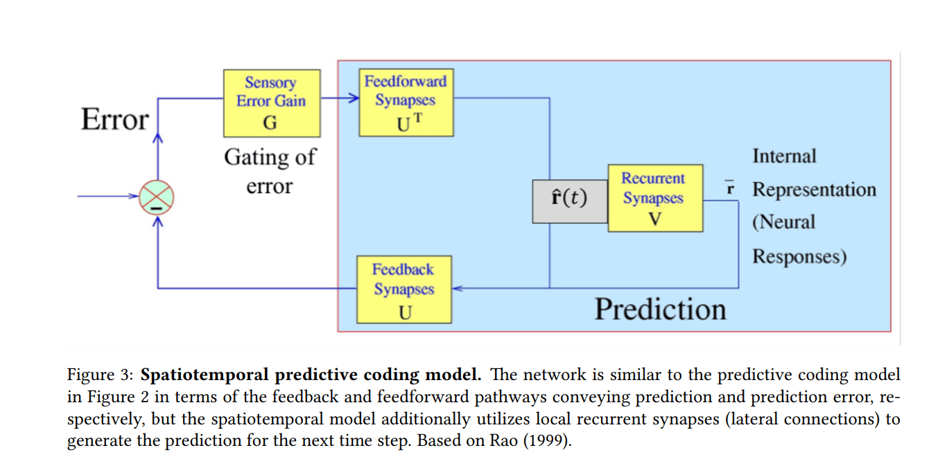
There are extensions to this model that deal with video, where there are explicit spatiotemporal expectations built into the network. you can see one of those networks in this paper: https://arxiv.org/abs/2112.10048
But I've never implemented such a network myself.
This is an overview of the classic 1999 paper by Rajesh Rao and David Ballard that introduced predictive coding. I'm going to focus on explaining the mathematical setup instead of just staying at a conceptual level. I'll do this in a series of steps of increasing detail and handholding, so that you can grasp the concepts by reading quickly, assuming you are familiar with the mathematical concepts. In addition I have implemented a convnet version of this framework in pytorch, which you can look at in this notebook:
Why I wrote this
The phrases "predictive coding" and "predictive processing" have squeezed their way outside of academia and into the public. They occur quite commonly on Lesswrong, and in related spaces. They are used to point towards a set of ideas that sound something like "the brain is trying to predict sensory input" or even more handwavy "everything about the mind and psychology is about prediction." This makes predictive coding[1] sound like a big theory of everything, but it was actually introduced into neuroscience as a very concrete mathematical model for the visual cortex.
If you are interested in these ideas, it is helpful to understand the mathematical framework that underlies the more grandiose statements. If nothing else, it grounds your thinking, and it potentially gives you a real mathematical playground to test any ideas you might have about predictive coding. Additionally, 1999 was quite a while ago, and in many ways I think the mathematics of predictive coding makes more intuitive sense in today's deep learning ways of thinking, than in the way originally presented. I've tried to port the original work into something that looks more at home in today's ways of thinking (e.g. the code on github i linked to implements a predictive coding network in pytorch and uses convnet structure etc.)
A note of clarification: there are other network implementations of predictive processing, but this is the original one that started everything. Karl Friston has said that this is the paper that led him to active inference.
A second note of clarification: My understanding of these terms is that predictive processing is an umbrella term that encompasses especially the more theory of everything type ideas, while predictive coding really refers to (a small set) of particular network architectures, like the one described here. But I do think people use these terms quite sloppily, even in academic literature.
Summary of the mathematical framework
Don't worry if this doesn't make sense to you right now, we'll be going through every piece. In order to get a predictive coding network we:
The Generative Model
The goal is to make a network that takes in images and represents the image in the activations of the network. More specifically, we think of the network as representing the causes of the image. For example, a cow is a physical object that exists out in the world. When we see a cow, photons bouncing off the cow hit our retina and our brains try to infer the physical setting of the world which caused the retinal image, i.e. a cow. We are not after a representation of the retinal image itself, but instead of the cow which caused the retinal image.
The retinal image we call I, and is represented as a vector of pixel values.
The causes of retinal images are given by a matrix U and a vector r. The columns of U are a basis for the causes. We think of r as the representation of a cause in the basis given by U. To spell this out a bit more, the numbers in r are the weights associated with each basis cause (i.e. each column in U), and the multiplication Ur is a linear combination of basis causes. There is also a nonlinearity, f, such that we assume images are related to causes in the following way
I=f(Ur)+n
where n is a noise vector that accounts for any error between the image and the inferred causes. We call this equation the generative model since it describes how causes in the world generate retinal images.
The rest of predictive coding (in the style of Rao and Ballard) is taking that generative model and applying Bayes Theorem to it, and then using gradient descent to maximize the posterior given a dataset. The gradient descent equations define a dynamics which are then interpreted as the dynamic activity of a recurrent neural network. And that's basically it! If you aren't interested in more detail or seeing the actual equations worked out, you can stop here, or skip to the simulation results.
A Fast Mathematical Tour from the Generative Model to Predictive Coding
A Simplified Non-heirarchical Version of Predictive Coding
Interesting terms in these equations:
Before we go into how these terms are interpreted as a recurrent neural network, let's extend the model to make it heirarchical.
Hierarchical Predictive Coding
Interesting terms in these equations:
Interpreting these equations as a recurrent neural network
We can visualize this hierarchical network as follows:
Hopefully by following the arrows and looking at the equation its pretty clear how the equations relate to the recurrent network. Here is a copy paste from a recent review by Jiang and Rao (2022).
More detail about the process
The setup is we are given a set of images (we will call a particular image I) and want to infer causes U over the dataset and an r for each image. We can use Bayesian inference to do this! Using the generative model, we can compute a likelihood - the probability of an image given causes, p(I|U,r). This is a distribution because of the noise term in the generative model. That is, given a particular setting of both U,r we still have a distribution over I because of the randomness of n. Ultimately we wish to find causes that maximize the posterior: p(U,r|I), in other words we want to find the causes that are most probable given an image. Using Bayes theorem we have
p(U,r|I)∝p(I|U,r)p(U)p(r)
Where p(U) and p(r) are priors on the causes. If we find the values of the causes that maximize the right hand side of the equation, we will maximize the left hand side. This is the approach we will take.
Computing likelihoods and priors
Remember the generative model has a noise term
I=f(Ur)+n
We assume that n is normally distributed with 0 mean and variance σ2, and with no covariance structure. Since normal distributions have exponents in them, we will take logarithms. The logarithm is monotonically increasing, so maximizing log(f(x)) is the same as maximizing f(x). Taking logarithms has the added bonus that the multiplication of the likelihood and the priors becomes an addition. By convention we like minimizing functions instead of maximizing, so we will also take the negative logarithm of our inference equation, and we will call that L:
L=−log(p(I|U,r)p(U)p(r))=−log(p(I|U,r))−log(p(U))−log(p(r))
We want to find U and r that minimize L!
I'm not going to go through the details of the math here, but using the equation for normal distributions we get the following form for L
L=1σ2|I−Ur|2+g(u)+h(r)
Where the functions g,h are the negative logarithms of the priors on U and r respectively.
Making the Network Hierarchical
We assumed that our generative model took the form of I=f(Ur)+n, which is to say that images are caused by causes. But what if those causes are themselves caused by more abstract higher-level causes, Uh and rh.
r=f(Uhrh)+nh
In this way, we treat the causes, r, of the retinal image as if it were sensory input to a more abstract system. This more abstracted system is trying to infer higher-level causes, rh in a basis given by Uh, of r. Now the overall posterior will be p(U,r,Uh,rh|I). As before, we can similarly derive an overall L
L=1σ2|I−f(Ur)|2+1σ2|r−f(Uhrh)|2+g(u)+h(r)+g(u)+h(r)
Finding r,rh,U, and Uh that minimize L will be the same as maximizing the posterior.
We can generalize this situation to add more levels to the heirarchy:
r0=f(U1r1)+n1
r1=f(U2r2)+n2
...
rm−1=f(Umrm)+nm
Minimizing L
Finding the representation of a specific image
To minimize L we will take derivatives and then use gradient descent, like one is used to in deep learning. Let's start with the gradient minimizing with respect to r.
dLdr=−2σ2UT(I−f(Ur))f′(Ur)T+2σ(r−f(Uhrh))+h′(r)
This equation is certainly a bit messy. Let's go through it slowly. The first thing that jumps out is the term, I−f(Ur). This is the difference between the actual image and the image estimated by the current setting of r. In other words, this is how much error there is between your prediction of what the image is based on your current guess of what the cause is, and the actual image, and so we call, I−f(Ur), the prediction error.
Similarly, r−f(Uhrh), is the error between the current setting of r and the prediction of r given by the higher-level causes. This is a higher-level prediction error.
Note that both the base-level and higher-level prediction error terms are (inversely) scaled by a variance term 1σ2, called the precision. The smaller your variance for the likelihood, the more precise the prediction error is, and so the relative contribution of that prediction error goes up. A lot of interesting ideas about how predictive coding is related to psychological phenomenon (e.g. mental illness) has to do with errors and manipulations of precision in the brain.
We have the following terms of interest, at each level of the heirarchy:
From the dynamical equation we can have a matrix -2/sigma2 U^T multiplied by the prediction error,
Note: I haven't finished this section but if you are following up to this point I think you probably get the idea. For the purposes of actually getting this out I'm leaving this as is, sorry.
Comparisons to standard deep-learning systems
Gradient descent is used to minimize loss in two ways
In the standard deep-learning setup gradient descent is used to find parameters of the network that minimize a loss function. The same thing happens in predictive coding networks, but it actually happens twice.
The first way gradient descent is used is the "normal" way - to learn features of the input that are useful for minimizing the loss. In our case this is how we change the parameters in the U matrices. These changes are computed over batches of many images.
The second way gradient descent is used is to find the activations of the neural network, in this case, to find the values of the r, given a single input image. This is not standard from the perspective of modern deep learning, but should set off mesa-optimizer alarm bells.
Training and inference are both dynamic
To expand on the previous point, in the standard case we use gradient descent for learning over a dataset, in other words for training our neural network. Thus, we can think of training as being a dynamical process. After that process, the parameters of the model are frozen and any new input can simply be run through the network to create an output. Thus, inference is simply a bunch of matrix multiplication and a few nonlinearities in a fixed network, and (usually) does not have much in the way of dynamics.
In predictive coding, inference is also a dynamic process. Even after training is over, for a given input image, we obtain the activations of our network by applying gradient descent dynamics.
We can think of training to be a long timescale process, and inference a short timescale process. While this is kind of the case in the standard setting, it only is in a trivial way, since standard inference usually doesn't have any notion of time or dynamics associated with it.
This is kinda sorta like an autoencoder
At least conceptually, though I do believe I've seem some work formally relating them, but I can't find the reference right now. In an autoencoder, you train the output to reproduce the input, after forcing all the input information through a bottleneck/latent space. In the predictive coding network, the network is, by virtue of its gradient descent dynamics to maximize the posterior, trying to reproduce the sensory input at the earliest layers of processing, via a heirarchical set of feedback connections which act as predictions. These predictions continually get refined by virtue of the recurrent dynamics in the network. It's like an autoencoder folded in on itself, with a bit more dynamics.
Some simple code/simulations
I've implemented a convnet pytorch version of this predictive coding network, which you can see in this notebook:
You can see the hyperparameters I've chosen in the model instantiation
The main ones are that there are 2 layers, with 8 basis causes in the first layer and 10 in the second, and that each cause in the first layer is a kernel of size 8x8 pixels, and each in the second layer is a kernel with size 3x3 (which is no longer in units of pixels but instead of first layer kernels).
With this we can train on a set of images, and then look at the input image, the prediction by the network (in the first layer, after multiple timesteps) and the difference, which I'm showing in the 3 columns of this figure:
One can also visualize the basis set in the first layer:
Obviously there's a lot more one can do. For instance, one can look at how the predictions change and converge over time, or can visualize predictions in higher layers, or can intervene on the network at higher levels in order to manipulate predictions from the top-down, etc.