Executive Summary

• I try vector-quantised autoencoders (VQ-VAEs) as an alternative compression scheme of transformer activations (as opposed to something like a sparse autoencoder).
  • Whilst people have danced around this idea before, discrete quantisation has only ever been tried in the actual transformer architecture itself, rather than on cached activations. 
• Specifically, I train a VQ-VAE on a data of 1000 cached model activations on the indirect objection identification (IOI) task (500 "positive" examples where the model is required to do IOI, and 500 "negative" examples where it isn't). 
  • For each forward pass through the model (i.e. for each example), this produces a sequence of n_layers discrete integer codes, supposedly capturing the semantics of that progression of the residual stream.
• I show that you can use something as simple as a categorical decision tree on these sequences of codes to extract very simple circuits from the model, and then examine the splits in the decision tree as a form of automatically interpreting this circuit.
  • I confirm that the "circuit" we found is quite close to the IOI circuit originally found in GPT-2 small, particularly since the whole process was unsupervised! Despite my current setup being very simplistic, I think that decision trees over these discrete codes can be a powerful tool for automated circuit discovery and interpretation.
• I extend the decision-tree circuit-finder/interpreter to the high-dimensional continuous residual streams.
• Finally, I briefly discuss how to make this whole process a bit more robust and how it might scale to more complex tasks and automated workflows.

All code for the VQ-VAE can be found here. All code for sampling can be found here.

Introduction

Mechanistic interpretability has recently made significant breakthroughs in automatically identifying circuits in real-world language models like GPT-2. However, no one has yet been able to automatically interpret these circuits once found; instead, each circuit requires significant manual inspection before we can begin to guess what is going on.

This post explores the use of compression in the form of autoencoders in order to make the residual streams of transformers acting on certain tasks much more conducive to automated analysis. Whilst previous groups have explored similar techniques for uncovering isolated features stored in specific layers (for instance, using sparse autoencoders and quantisation), no-one (to my knowledge) has yet determined whether these compression schemes can be applied across layers sequentially. By looking at the residual stream as we move through the layers of a pre-trained transformer, and using a clever compression scheme, we might be able to capture how computation is represented in consecutive layers, from input to output logits.

The appeal of employing Vector-Quantised Variational Autoencoders (VQ-VAEs) in the analysis of transformer-based models lies in the advantage (I believe) of discrete quantisation over continuous compression methods such as sparse autoencoders. By converting high-dimensional, continuous residual streams into discrete codes, VQ-VAEs offer a simplified yet potent representation that is inherently easier to manipulate and interpret. This quantisation process not only aids in identifying computational motifs across layers of a transformer but also facilitates a more straightforward understanding of how these layers interact to perform specific tasks like IOI. Unlike methods that focus on isolated features within static layers, the sequential nature of VQ-VAE compression captures the dynamics of computation through the transformer architecture, presenting a holistic view of model processing. This characteristic makes VQ-VAEs particularly suitable for tracing and interpreting the computational paths—'circuits'—that underlie model decisions.

To be honest, I didn't really know what I would do with these quantised residual streams once I had them. However, after playing around a lot with training simple probes to distinguish between positive and negative examples of the IOI task (and look at correlations between codes, etc.), I realised that none of what I was doing was scaleable (we required a human to interpret and the labels). Thus, none of what I was doing was automatable, which was the idea of having these codes in the first place. I realised that I needed an approach that would simultaneously determine what codes were important in the particular task, and also what these codes were actually representing.

This is where I came up with the idea of using a decision tree to do both of these at once. I one-hot-encode all n_layers dimensions of the quantised sequences representing the residual streams, and then train a decision tree on this categorical data. The cool thing about decision trees is that they choose the features (in our case, the codes) that minimise the entropy of the splits i.e. achieve maximum separation between positive and negative IOI examples. Not only this, we can directly look at these splits to determine which codes in which layers are the most important, and how they affect the final decision. 

Whilst my analysis is quite simple and performed on a well-known circuit, I'm fairly confident there's enough evidence here to suggest making this approach more robust might be a valuable thing to do. Whilst this work was done in a big sprint over only a few days, I'm currently trying to scale my technique/s to more algorithmic datasets and general activations cached from forward passes on the Pile.

Collating a dataset and training the VQ-VAE

Indirect Object Identification (IOI) Task

The Indirect Object Identification (IOI) task is designed to evaluate a language model's ability to discern the correct indirect object in a given sentence structure. The classic example given in countless TransformerLens demos is "When John and Mary went to the store, Mary gave a bottle of milk to ", and the model is tasked with correctly predicting "John" rather than "Mary". The task's objective is to predict that the final token in the sentence corresponds to the indirect object. This setup not only probes the model's grasp of syntactic roles but also its understanding of semantic relationships within sentence constructs. The challenge lies in correctly identifying the indirect object despite variations in sentence structure and the presence of distractor elements (e.g. whether the subject of the sentence comes first or second in the initial list of names). 

In the context of GPT-2 small, the IOI task serves as a litmus test for the model's linguistic and contextual comprehension. By generating sentences through predefined templates and measuring the model's performance with metrics such as logit difference and IO probability, researchers have quantitatively assessed GPT-2 small's proficiency. Impressively, across over 100,000 dataset examples, GPT-2 small demonstrated a high accuracy in predicting the indirect object, with a mean logit difference indicating a strong preference for the correct indirect object over other candidates (Wang et al. (2022)). 

Since we know that GPT-2 can perform this task, we know that somewhere in the computation ledger of its sequential residual streams, it's focusing on the names and how to predict the indirect object. We want to take these high-dimensional continuous residual streams and compress them to a sequences of discrete integer codes, which we will do with a VQ-VAE.

Vector-Quantised Autoencoders (VQ-VAEs)

Vector-Quantised Variational AutoEncoders (VQ-VAEs) introduce a discrete latent representation into the autoencoder paradigm. At its core, a VQ-VAE comprises an encoder, a discrete latent space, and a decoder. The encoder maps an input $x$ to a continuous latent representation $z_e\left(x\right)$. This representation is then quantised to the nearest vector in a predefined, finite set $Z=\{z_k{\}}_{k=1}^K$, where $K$ is the size of the latent embedding space, forming the quantised latent representation $z_q$.

The quantisation process transforms $z_e\left(x\right)$ into $z_q$ by finding the nearest $z_k$ in $Z$, effectively compressing the input into a discrete form. The decoder then reconstructs the input from $z_q$. This setup introduces a non-differentiable operation during quantisation, which is circumvented by applying a straight-through estimator in the backward pass, allowing gradients to flow from the decoder back to the encoder. Additionally, to maintain a rich and useful set of embeddings in $Z$, VQ-VAEs employ a commitment loss, penalising the distance between $z_e\left(x\right)$ and $z_q$. This stops the volume of the embedding space from growing arbitrarily and forces the encoder to commit to an embedding. This architecture enables VQ-VAEs to learn powerful, discrete representations of data.

As noted in the introduction, our aim is to apply the VQ-VAE to collections of the sequence of residual streams obtained from individual forward passes through a transformer model on the IOI task. Since GPT-2 small has a model dimension of 768, and there are 13 layers (including the embedding and output; 26 if we break it down by attention block and MLP block) and we will have n examples, the VQ-VAE will help us take a sequence of size (n_layers, n_examples, d_model) to one of size (n_layers, n_examples). Each layer in the residual stream will be assigned a single "code" from the codebook that best represents the computation being undertaken in that specific residual stream. The aim is to see whether analysis of these codes can do some or all of the following:

• Distinguish between when the model is doing IOI vs. when it isn't
• Determining which components of the model (i.e. which attention and MLP blocks in which layer) are important for the model in performing the IOI task
• Interpreting these codes in the context of circuits (a path/subgraph) through the layers of the model rather than typical code-style analysis which looks at isolated, static features

There's notoriously a lot of tricks involved in training a VQ-VAE. For instance:

• Using a lower codebook dimension
• ${\ell }_2$ normalising the codes and the encoded vectors (this paper claims that forcing the vectors to be on a hypersphere improves code usage)
• Expiring stale codes
• Forcing the codebook to be orthogonal, meaning translation equivariance of the codes
• Various different additional losses

These are basically just ways of (1) getting the codes to be more meaningful, and (2) getting the autoencoder to use more codes. There have been proposed alternatives to VQ-VAE, including Finite Scalar Quantisation (FSQ). Although this drastically simplifies the autoencoder, I found the ability to expire stale codes to be quite useful when training my VQ-VAE, so I stuck with it. As I've noted in the conclusion, I'd like to implement expiring stale codes for FSQ in the future so I can simplify my autoencoder's bottleneck.

Determining importance and presence of meaning in quantised streams

As a prelude to all the analysis, the basic steps I went through were:

1. Collect a dataset of 500 examples of positive IOI examples using Redwood Research's excellent EasyTransformer code. We hereon refer to these as "positive" examples of the IOI task
2. Collect a dataset of 500 "negative" examples where the model was not required to do IOI analysis. I initially got these 500 examples from randomly sampling the Pile but later realised this was stupid and switched to negative examples where there were simply three names in the IOI sentence e.g. "When John and Mary went to the store, Charlie gave a bottle of milk to ". However, until we get to that section, just assume that a negative example comes from the Pile i.e. a random sentence from the internet. 
3. Tokenise all these prompts and run GPT-2 Small on them, caching the residual streams for the last token (i.e. the one where we either need to do IOI name prediction or not). This gives a dataset of 1000 residual streams, each of size (n_layers, d_model) = (13, 768). In another stupid move, I initially used the accumulated residual stream for this, which "can be thought of as what the model “believes” at each point in the residual stream" (see the docs). This is because I was thinking of the residual stream as a computational ledger. However, if you want to assign a code to different layers of any given residual stream in isolation like we're doing here, you care more about the decomposed residual stream, which basically looks at what individual components (attention and MLP blocks) are doing. Again, until we get to the point where I realise this mistake, just assume I used accumulated resid. (You could also probably take the difference between consecutive residual streams as another way around this; I've put this on the to-do list for future in the conclusion). 
4. Train our VQ-VAE on a random split of examples and their residual streams. Using a training size of 80%, we get a 13x800x768 sized tensor for our training samples, and a 13x200x768 tensor for our validation examples.
5. Train until we get pretty loss pretty low (scientific, I know). 

Unsupervised evidence

This is just a small collection of initial evidence I looked at to confirm the codes used to represent positive examples and negative examples were indeed different. Although there is no notion of order among these latent codes (they are categorical), just plotting the mean positive indices across all 500 positive examples minus the mean negative indices across all 500 negative examples reveals a big difference, particularly in later layers.

Although it doesn't necessarily make sense to do this, PCA of the codes reveals some separation (just in the codes, not the residual streams) between positive and negative code sequences:

This is perhaps more obvious if we plot the mean code at each layer by positive and negative:

So we've clearly learned some representation that distinguishes between positive and negative IOI examples. But what exactly have we learned?

Decision trees

My first idea was to take all the indices and simply train a decision tree to predict whether a particular sequence of 13 codes was positive or negative. Decision trees are really handy for this interpretability analysis, I reasoned, because you can easily access the "splits" the model made at each decision node in order to reduce the entropy of the splits (i.e. which features are most informative in predicting a positive or negative example). I initially tried this on all the codes, and got a test accuracy of 93.5%. That's good! I could also draw the decision tree's decisions:

In all honesty, this isn't very interpretable. Whilst we get good accuracy of 93.5%, the tree is too deep to interpret what is going on. What if we set the max depth of the decision tree to just two (corresponding to two layers of splits) to basically enforce interpretability? Amazingly, our accuracy only drops a miniscule amount, to 93%. And our decision tree is now extremely interpretable:

This is a great finding! We get an accuracy of 0.935 with a max depth of 17, and an accuracy of 0.93 with a max depth of 2. This means that our quantised codes have found a meaningful way to represent the task at hand with basically one code! It looks like the 12th code (i.e. the final layer) is the important thing here (the DT chooses to split on it twice). Let's dig in to the difference between positive and negative examples in the 12th layer.

The first thing we'll do is calculate the PCA of the 12th layer residual streams, and colour them by whether they're positive or negative. Interestingly, PCA creates a linear separation between positive and negative IOI residual streams.

I now believed I was onto something with the decision tree analysis, and so I wanted to extend it to more meaningfully analyse individual codes, rather than just the layer where those codes occurred.

Categorical decision tree

So to summarise where we're at: we have some clearly meaningful sequences of discrete codes that represent the sequential residual streams of a forward pass through our transformer models. That is, we assign one token per residual stream (a vector of size 768, the model dimension) at each layer, resulting in a sequence of 13 tokens per forward pass. 

We have shown that these codes are meaningful at distinguishing when we're doing the IOI task versus not with a bunch of evidence. A decision tree classifier trained on the indices obtains an accuracy of 93% with a maximum depth of two. We also see that there is very little overlap in the codes when the model is IOIing and when it's not. Finally, we see that the difference in codes between doing the task and not can be isolated to specific layers. For instance, a PCA of the layer residual streams creates a linear separation between positive and negative IOI streams.

However, decision trees aren't the best option for automatically interpreting these sequential codes. This is largely because they can only "split" the data on some threshold of some feature (i.e. a given layer's code) and thus treats codes like continuous features rather than categorical features like they really are. 

An obvious solution to this is one-hot encoding the discrete codes from each layer before feeding them into the classifier. By converting each unique code into its own binary feature, we ensure that the model treats these codes as separate entities rather than attempting to interpret them along a continuous spectrum. This is crucial for our analysis because each code represents a distinct "category" or "state" within the residual stream of the transformer model, not a point along a numerical scale. Rather than splitting on a threshold value of a feature, the classifier can now leverage the presence or absence of each code across the layers, reflecting the true nature of our data. This approach aligns with our understanding that the sequences of discrete codes carry meaningful distinctions between when the transformer model is engaged in the IOI task and when it is not.

After one-hot encoding our features and training a decision tree, we get a test accuracy of 100% with a tree depth of just 6. Recall that we're now using one-hot encoded vectors, so a tree depth of 6 means we can distinguish between positive and negative IOI examples just by searching for the presence/absence of six individual codes.

A great thing about decision trees is that we can plot the feature importances. In decision trees, feature importances are calculated based on the reduction in impurity or disorder (measured by Gini Impurity or entropy) each feature achieves when used to split the data, quantified as information gain. This gain is aggregated and normalised across the tree to reflect each feature's relative contribution to improving classification accuracy. So in our case, feature importances are simply the codes the DT found most informative for distinguishing between positive and negative examples. 

Note: to get the feature names I created a mapping between the one-hot encoded indices matrix and the layer + code.

This gives us what we need next: the particular codes in the particular residual stream that are most informative in distinguishing positive and negative examples. Now, we need to figure out exactly what these codes mean, how the sequential interplay between codes affects computation, and whether it's possible to leverage the code sequences for automatic interpretation.

Determining actual meaning of quantised streams

I think at this point it's useful to do a brief literature review of how people find meaning in latent representations of model activations. There are probably two key papers that cover ~95% of the relevant approaches here (of course, Anthropic has gone into further depth, but you can read about that in your own time). 

Tamkin et al. (2023) trained a quantiser inserted in between layers of an existing transformer, and then used these intermediate code activations as a base for interpretation. Interpretation was a combination of static and causal analysis. First, they found that most codes were activated infrequently in the training activations, and so they could get a rough idea of a code's function by looking at the examples where it activated (this is very common). As I note in the conclusion, quantising has an advantage over continuous representations here because it is discrete and prevents neurons "smuggling" information between layers. They also show that replacing codes in intermediate representations during the forward pass allows you to inject the topic associated with that code into the sampled tokens in a natural way. They measure the success of this by using a simple classifier. 

In a similar line of work, Cunningham et al. (2023) train a sparse autoencoder on a static dataset of activations across a chunk of the Pile. (In contrast to the above, they train it on cached activations outside the model, rather than inserting the autoencoder into the model itself and then training that.) They then use autointerpretability to interpret learned dictionary features: looking at text samples that activate that feature, and then prompting an LLM to interpret the feature and predict the dictionary feature's activation on other samples of text. "The correlation between the model’s predicted activations and the actual activations is that feature’s interpretability score." 

They also do some causal analysis by using activation patching. Basically, they edit the model's internal activations along the directions indicated by the dictionary features and measure the change to the model's outputs. Doing so with dictionary features requires fewer patches than a PCA decomposition. Other analyses include:

• Plotting histograms of dictionary feature activation across token activations to show a separate of histograms and thus monosemanticity
• Subtracting a dictionary feature's value from the residual stream and seeing if it has a logical effect on the next token prediction; for instance, subtracting the apostrophe feature reduces the logit for "s"

Perhaps the most relevant of all techniques is their analysis of which dictionary features in previous layers cause a specified feature to activate. This is closest to the circuit-style analysis that we're looking to perform on our sequences of codes. The process involves selecting a target feature, identifying its peak activation, and then selecting 20 contexts that activate it within the range of half its maximum $M/2$ to its maximum $M$ activation. For each feature in the preceding layer, the model is rerun without (ablating) this feature, and these features are ranked based on the extent to which their removal reduces the activation of the target feature. This method can be recursively applied to significantly impactful features in prior layers to trace the activation pathway back through the network.

Given all this, we're going to pursue some similar style analyses. 

Manual interpretability for most common codes

By using the feature importances from our pre-trained decision tree, we can look at the frequency with which the most common codes occur in positive examples. There's quite a few that stand out. For instance, code 459 occurs in over 40% of our positive examples.

This begs the question of whether there is additional structure in the other codes that is representing some differences in our IOI task, or whether we just trained a VQ-VAE with too many codes (i.e. because we were too quick to expire stale codes). To answer this question, the easiest thing I could think of to do was embed the prompts with something like ada, calculate the PCA, and colour by code. 

Doesn't look like much signal there. Additionally, I trained a logistic regression model on the embeddings to see if we could predict the associated code, and got a test accuracy of 40%. Whilst this is better than chance (there are six classes), it's not great, and unlikely to distinguish between anything meaningful. 

Of course, we can also check for algorithmic patterns e.g. whether one code is when the indirect object comes first or second in the initial names. For reasons outlined below, I leave this to a future analysis. 

Circuit backpedalling

I then had a whack idea. What if you applied the decision tree thing all the way down? That is, predict which codes are most important for predicting positive vs. negative. Then, use a decision tree to predict which codes in the previous layer are the most important for predicting the predictive code. And just go back recursively through layers until you have a "circuit". 

In other words, I used a DT classifier to iteratively identify and rank the significance of features based on their contribution to the binary classification task of predicting a positive or negative IOI example. Starting from the ensemble of one-hot encoded features, each iteration zeroes in on the most pivotal feature, as determined by the classifier. Upon identifying this key feature, we then dynamically update our target labels to be the presence or absence of this feature's specific code across our dataset examples. We then predict which codes in earlier layers are most important for predicting the current feature. Through this method, layer by layer, we arrive at a "circuit" of the most significant features and their contributions to model predictions.

When running the circuit finder, we get the following circuit.

I then did a bunch of rather uninteresting analyses. For instance, in looking at the collection of all indices from all examples, all of the 15 examples "closest" to the circuit (defined by how many codes they share with the circuit in the specified layers) were all positive. However, without looking into exactly what each residual stream is doing (in the original high-dimensional space) at each layer, it's a bit hard to make any more progress. I dive into this a bit later on.

Replacing residual streams with ablated discrete representations

The next thing I wanted to play around with was taking the circuit found above and seeing what outputs GPT-2 would produce from the reconstructed residual stream. To do this, we take the codes in the "most important" circuit found above, insert randomly sampled codes at layers where there wasn't a code in the circuit, and reconstructing the residual streams using the decoder from our model above. 

Note: since we're using the trick where we project down our quantised vectors in the VQ bottleneck, we need to remember to project them back out before we can decode them. See the Github, but essentially this amounts to:

low_dim_vectors = model.quantizer.get_codes_from_indices([indices])
quantized_memory = model.quantizer.project_out(low_dim_vectors)

Once we have our reconstructed residual stream, we can then do the typical logit lens-style analysis on our residual stream. We take our reconstructed residual streams, apply a layer norm to each (as GPT-2 expects a final layer norm), and project them back out with the unembedding matrix $W_U$. For a start, this gets us the predicted token when we unembed each layer.

So once we get to the final residual stream, we predict a name. Okay, so our circuit has found something, but probably not too interesting until we get to the final layer. It's also interesting to look at the top 10 tokens from the final layer:

All names. So the 459 code in layer 12 is likely just signalling "There should be a name here". What happens when we corrupt this and replace it with a random code from the negative examples?

What this tells me is that basically the only salient code for our specific task is the one in the last layer that says "We need to predict a name". This is a start, but it's not exactly ground breaking. Let's see if we can find something more circuity (i.e. interplay between layers) and algorithmic.

Retraining and regrouping

Changes to the setup

Noting all of my above mistakes and results of the analysis thus far, we're going to make some small but significant changes to our setup:

• Instead of our "negative examples" being drawn randomly from the Pile, we're going to make them similar to the IOI examples but with the indirect object hint being neither of the two previous names. For instance, if the positive example is "When John and Mary went to the shops, Mary gave a bottle of milk to", then the negative example would be something like "When John and Mary went to the shops, Charlie gave a bottle of milk to". Rationale: if we have negative examples closely aligned to our positive examples except in small, patterned ways, the VQ-VAE will be "forced" to spend codes differentiating the two.
• I didn't actually train my previous VQ-VAE until convergence, so now I will. This will also involve optimising things like the number of codes, the number of encoder/decoder layers, the codebook vectors projection down, and several other choices. Rationale: if the loss is basically zero, then the codes will have to be meaningful enough to capture the differences between these positive and negative examples. Since we know GPT-2 is able to distinguish between the two cases, if our VQ-VAE is good enough and is trained for long enough, it should be able to as well, which will facilitate circuit-style analysis of our codes.
• I'm going to shrink the number of codes as much as I can without compromising performance too much. Rationale: by only having a few codes, again we force the model to capture the key parts of its thinking, which is hopefully what name comes next.

Training and ablation studies

Final train and eval losses followed each other very closely:

I wanted to make sure the final reconstruction loss was as low as possible so I did Bayesian hyperparameter optimisation with Optuna:

Interestingly, the most important hyperparameter was commitment weight:

But in all honesty, the final eval loss didn't really change at all. I'm guessing you'd see the eval losses plateau for smaller codebook sizes with more training, but training this long makes it difficult to optimise in Optuna due to compute constraints. Also, the loss for all of them is quite low overall anyway.

Number of encoder and decoder layers

The last thing I wanted to check was how the depth of our autoencoder affected the final loss. 

Seems to be instability in training as we increase the number of layers. Not much more to look into there without getting into the depths of our architecture, which I don't want to waste time on for the moment. The final values of hyperparameters (relating to the quantiser) were:

• Codebook size = 32
• Codebook dimension (projected down) = 16
• Threshold EMA dead codes = 2
• Commitment weight = 1.0
• Decay = 0.8

Code circuit analysis

I'm then froze my model weights and considered it trained. Again, we got the discrete bottleneck representations of all examples as indices, and trained our categorical decision tree to predict positive from negative IOI examples.

We get an accuracy of 89% with a DT depth of 5. This is good - even with only 32 codes and positive and negative examples that are much semantically closer, we're good at distinguishing between the two cases just by looking at the discretised code sequences. Let's have a look at the important codes. 

Layer 18 (corresponding to attention layer 8) looks extremely important. I'll do another PCA to see if it separates the positive and negative examples.

It's definitely separating it heaps! I checked the layer before (and a few others I haven't included) to ensure that not all layers are doing this separation:

Definitely not! There's something special about layer 18. Now we've found that the most important layer is 18 (corresponding to attention block 8), we need to confirm that this attention block is actually doing something for the task. The best way to do this is get some corrupted activations (i.e. where the model is not doing the IOI task, or is doing it differently) and then intervene by patching in specific clean activations from a clean prompt (where it is doing that task). If you define a metric of how close to the "correct" answer it is (i.e. the logit difference of the correct token and another plausible token), then you can figure out which components of the model are important for getting the correct answer on the specific task.

We initially keep this simple and just look at 8 IOI prompts covered in the IOI analysis tutorial. Our metric is the logit difference between the subject and indirect object's name (should be high if we're doing well). After applying activation patching to the residual streams after attention blocks, we get the following plot:

As we can see, the attention layer 8 has the largest positive contribution to the logit difference. As Neel Nanda notes in his exploratory demo, "[presumably this the head] that moves information about which name is duplicated from the second subject token to the final token."

Can we go one step further and see if we can isolate index 481 in the residual stream of layer 18 (attention block 8)? I haven't quite figured out how to do this yet, but I'm currently trying out some ideas. I think it's definitely possible, but requires decomposing the residual stream further into specific heads.

So summing up, our most important code found an S-Inhibition head, named so due to the original IOI circuit paper. These output of these heads is used to inhibit the attention paid to the other name in the sequence. 

So why did we find this particular head? Well, if you think about the new prompts we looked at, it actually makes the most sense. We're now examining "corrupted" prompts just with the names switched order. We're not using our counterexamples we trained the VQ-VAE on. So, the most important discrete latent code for distinguishing between positive IOI examples and the negative examples (where we used a completely different third name) would be a code that signifies whether we're suppressing the direct object (the repeated name) or not. Whilst this evidence is only circumstantial, I think the evidence from the above paper makes it fairly likely that this is what our VQ-VAE has learned to represent with code 5 in layer 18. 

Using our actual counterexamples

The last thing we want to do here is repeat our above analysis with the corrupted examples that more closely resemble our original negative examples. That is, the third name (the direct object) is replaced with a name that is neither of the first two names. We can then recalculate the importance of each attention layer in predicting the correct token. By subtracting the importance of each layer obtained from patching with the original corrupted examples above, we see that our good old attention layer 8 has the highest difference!

Interpreting this, we see that attention layer 8 matters on both tasks, but it matters the most when the corrupted examples do not require S-inhibition. This is further evidence that attention layer 8 is doing S-inhibition and even cooler shows that our VQ-VAE is learning the "right" representations of the residual stream. 

Note: we're still using the logit difference from before, which is a bit hacky. I guess you could just use the logit difference to the next highest-ranked name in the logits (since there's no natural "other answer") but I didn't try this.

When I extend on this, I'm going to apply the same analysis to the other important layers found above (mainly 19, 20 and 10). I think layer 10 in particular (attention layer 4) is could be doing a lot of computation on the second subject token, (maybe figuring out whether it's repeated or not), and then later layers are moving this information to the final token. 

For reference, here's the "most important circuit" we found in the new quantised sequences with our categorical decision-transformer circuit finder, translating the layers to the actual layer names in the decomposed residual stream:

Let's compare this circuit to the one found by the original IOI paper: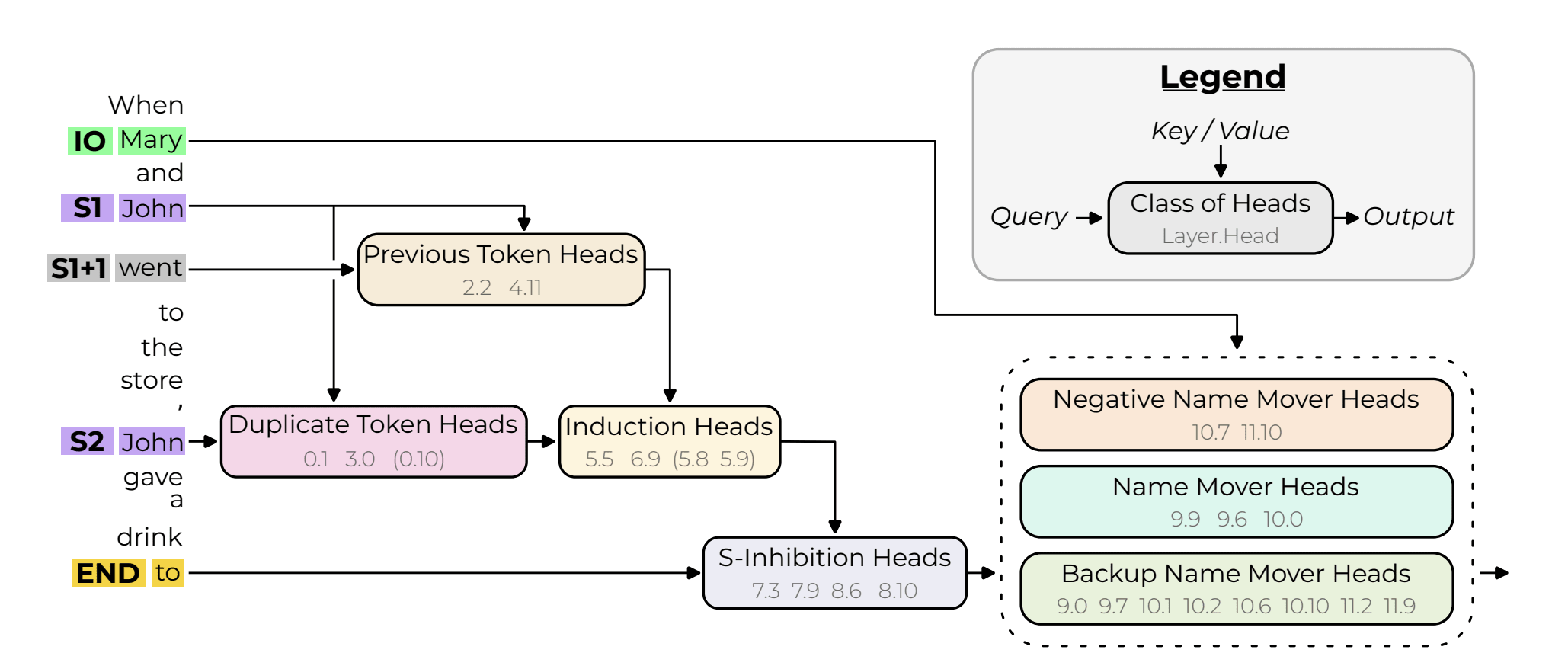

Our automated decision-tree circuit finder has picked up on the layer 7 and 8 S-inhibition heads. It also seems to have picked up on the duplicate token heads in layer 3 and 0 (embed). Finally, it got one of the previous token heads (2). (When I say heads, I mean the attention layer that contains the heads found in the original circuit.) We missed some induction heads and backup name mover heads; this is also sort of expected, as you miss both of these when doing the exploratory analysis tutorial in TransformerLens. However, overall this is promising! With no supervision, we got a lot of the important components of the actual circuit. 

And when you think about it, it makes sense that we didn't get all the components. Because we restrict our circuit to be what amounts to a one-input, one-output feedforward circuit, we're going to miss inter-layer interactions and more complex circuits. I think the fact we recovered this percentage of the IOI circuit is cool and suggests this methodology might hold value for automated circuit discovery and interpretation.

Of course, we could have just got lucky. However, there's 26 layers overall. We didn't select any MLP layers, and all 6 layers we selected contain a head named in the original circuit. What's the probably of doing this by chance? If you simplify the problem somewhat (read: extremely) and determine the likelihood of randomly choosing 6 layers containing a "correct head" from a total of 24, with 8 layers actually containing these heads, you get approximately 0.0208%, indicating the rarity of such a selection occurring by mere chance. (Don't come at me, I know how many simplifying assumptions I made with that probability.)

Extending on the decision tree as a circuit-finder

Can we use our decision tree method on the actual residual streams in order to find the same IOI circuit as previous papers? I think we definitely can.

Implementation

To adapt the original discrete token-based analysis to the continuous, high-dimensional residual stream data, I had to change a few things. Initially, the residual streams were reshaped from a 3D tensor to a 2D matrix to create a flat vector for each example. We transitioned from using a decision tree classifier for all iterations to employing it only for the initial iteration to determine the most critical binary distinction between positive IOI examples and negative. Subsequently, a decision tree regressor was used for continuous prediction of feature values, reflecting the shift from discrete to continuous data handling. The pseudocode is below:

resid_streams_flat = reshape resid_streams to 2D matrix
labels = concatenate equal parts ones and zeros
X_train, X_test, y_train, y_test = split resid_streams_flat and labels for training and testing
feature_importance_circuit = []
first_iteration = True

# Main loop for feature importance analysis
while True:
    # Select model type based on iteration
    if first_iteration:
        model = DecisionTreeClassifier()
    else:
        model = DecisionTreeRegressor()

    # Train model on current data
    model.fit(X_train, y_train)

    # Obtain and analyze feature importances
    importances = model.feature_importances_
    most_important_feature_index = index of maximum value in importances
    layer_index = most_important_feature_index / 768
    position_within_layer = most_important_feature_index % 768

    # Append layer and position to the circuit list
    feature_importance_circuit.append((layer_index, position_within_layer))

    # Break loop if the first layer is reached
    if layer_index == 0:
        break

    # Update targets with values of the most important feature if not first iteration
    if not first_iteration:
        y_train = values of most_important_feature_index from X_train
        y_test = values of most_important_feature_index from X_test

    # Exclude features from the identified layer and higher
    X_train = X_train[:, :layer_index * 768]
    X_test = X_test[:, :layer_index * 768]

    # Set first_iteration to False for subsequent iterations
    first_iteration = False

A significant modification was the dynamic update of targets based on the most important feature identified in each iteration, directly aligning the model's focus with the iterative discovery of the feature importance circuit through the transformer layers. This necessitated updating target values before excluding features for the next iteration to avoid indexing errors. Features from the identified important layer and higher are excluded in subsequent iterations, narrowing the feature space to those preceding the identified important feature. This process iteratively constructs a circuit of feature importance through the model, starting from later layers and moving towards the initial layers, culminating in a mapped circuit of the most influential paths through the transformer's architecture.

When running the above algorithm, we got the following circuit:

Interestingly, it's quite different to the circuit obtained on the discrete codes, and definitely not as aligned with the layers found in the original IOI paper. This suggests that the VQ-VAE might be learning a good representation that something like a decision tree can't extract from the high-dimensional continuous vector space of residual streams. Interestingly though, the same indices appear quite a few times in this circuit (corresponding to specific positions in the residual stream). I think it would be a good next step to look at what's going on in these positions and whether we can interpret them. 

Conclusion

I have a bunch more things to try/am currently working on:

• Determine the difference between the two groups in PCA of codes that are positive (e.g. is it first name first or second name first)?
  • The point here is to find some tokens that represent different patterns in the positive IOI examples e.g. ABA or ABB or ABC (I think you could automate labelling of these, look at clusters, assign codes, etc.)
• The fact that VQ-VAEs construct a discrete representation as opposed to a continuous one from sparse autoencoders means we can apply the decision tree layer analysis directly. This means we should probably train a big VQ-VAE on a bunch of activations and do some automated analysis. I'm currently collecting a big dataset from the Pile (much like this paper) to train a VQ-VAE on. I will open-source this once I'm done.
• Our VQ-VAE is forced to assign just one token to each residual stream. What happens when you assign multiple tokens per residual stream? Does this greater expressiveness make it easier or harder to interpret?
• Distinguishing multiple different tasks i.e. can it tell when we're doing docstrings, the greater-than task, etc.
• I'd like to do the whole thing on an algorithmically-designed dataset, which is almost conducive to being represented by discrete codes.
• In order to remove the stateful nature of residual streams across layers, repeat the whole analysis on differences in residual streams across layers.

In general, I'm pretty excited about using VQ-VAEs as a compression scheme for interpretability. I think discrete representations, which can be handled by transformers, make things a lot easier. In conjunction with my automated decision tree circuit analyser (which as far as I'm aware is novel), this could be a powerful tool in the mech interp toolbox.