A direction can be interpretable, causal, and predictive (and still a bad handle for intervention)
TLDR: In modern interpretability, we find “directions” inside a language model that seem to encode meaningful concepts. One such example is “This is about food.” A common next step is to steer the model in that direction, in the hopes it produces more of that concept. I show that even when a direction passes the tests we have for whether it “really” means something, the range over which the idea of “more pushing = more concept” remains valid is smaller than is often made explicit in steering work. I derive a closed-form, local Taylor formula that gives a radius within which the quadratic and cubic corrections are bounded relative to the linear term. Empirically, this radius predicts where steering stops behaving linearly across the models I tested. At , the linearity test failed in the median evaluated cell on 92% of inputs.
A direction in a language model’s residual stream—a vector within the information passed between layers—can be interpretable, causally relevant, and predictive of next-token loss, and still give an incredibly small radius inside which the linear reading of the edit survives! The gap between understanding the direction and how hard it can be pushed is what I set out to answer.
Papers tend to use which just means “multiply the direction by 1 and add it back to the models’ hidden state. I pushed along this track and found that the model’s behavior change stopped tracking this story long before I even reached
What’s actually going on when you push
Picture the model’s hidden state as a very high-dimensional vector. A steering direction is just another vector in the same space. To intervene in the model, you add some multiple of said steering direction (this is the I previously mentioned) to the hidden state, then run the rest of the model and see how the output changes.
For very small , push gently, and the model’s output change is roughly linear in: double the push, double the effect. This is what I call the "linear steering story". In other words, this direction encodes concept X, so pushing it makes the model do more of X, in proportion to the push. Many steering results are motivated using this linear reading.
For a larger the story doesn’t hold. The model’s behavior keeps changing. Sometimes a lot, sometimes hardly. But it stops being proportional. Quadratic and cubic effects creep in, and the linear idea of “more in more out” loses its grip on reality.
My question: how far can go before the linear story fails?
I found the answer involves three local properties of the direction.
1. How steep the loss landscape is along the direction
2. How curved it is along the direction
3. The magnitude of the third directional derivative
Call those 3 numbers, Each one costs about one autodiff pass to compute. Plug them, plus a tolerance into one formula
Plug in and your tolerance, and out comes . This is the largest push you can apply before the higher-order corrections (the quadratic/cubic terms) outgrow the tolerance the linear effect. To be clear, it does not, by itself, bound everything past cubic in the real model; it is a conservative radius inside which the quadratic and cubic terms of the Taylor approximation are bounded relative to the linear term. At my default tolerance of 0.5, that's the largest push at which the higher-order corrections are still less than half the size of the linear effect.
To take a step back and look at where this comes from. Taylor-expand the loss along the direction, drop everything past cubic, and you get three terms:
The story ultimately supports the claim that the first term dominates. Set the magnitude of the quadratic and cubic terms equal to times the magnitude of the linear term, solve for , and the formula above comes out. When the quadratic and cubic terms cancel, the formula is conservative rather than the largest possible radius.
Two different directions with the same get the same , no matter what method you used to find them. This tells us that it isn't a fact aboutsparse autoencoders,attribution patching, or whatever method gets a spotlight at the next conference. It is a fact based purely on the geometry of the direction itself.
Does it actually work?
I ran this diagnostic on eight language models across four families and four size orders:Qwen 2.5at 0.5B, 1.5B, and 3B;Gemma 2-2B;Pythia at 160M and 1.4B; and two non-transformer models,Mamba1-130M andMamba2-130M. I used 120 inputs per model, seven direction-finding methods, and a random direction baseline as a check.
For each direction on each input, I computed two numbers: the formula’s prediction and the measured linearity radius. The maximal safe push is the largest where the story remains supported in real tests; I call this . is an empirical companion to the formula. The question is whether the formula’s predictions () align with these measurements ().
It does, on every single model tested. The correlation between predicted and measured safe push ranges from 0.49 to 0.80 across the models, rising from 0.52-0.93 in the positive-sign subset. These are correlations on the resolvable examples.
At , across 43-evaluated model-layer-method cells, the empirical story test fails on between 52% and 100% of inputs. The median cell is 92% broken. Extending the same summary across all eight model datasets gives a range of 38.8% to 100% and a median of 89.2%. is more often outside the story’s regime than inside it.
Same Idea, Different Tool
If the breakdown really comes from local loss geometry (and not from which method you used to find the direction), then a different first-order interpretability tool should show related failures when the local-linear approximation breaks.
Attribution patching is one such tool, popular as an alternative to direct intervention. Instead of running the full counterfactual activation intervention and measuring the resulting change, you approximate the effect using only the first-order term (the gradient, which indicates how the output changes with small parameter adjustments). This first-order term underpins the method. The method, therefore, assumes higher-order corrections remain small. My proposed formula gives a diagnostic on where the assumption breaks.
Across three model families, on every combination of model and layer where I had a clean enough signal to estimate, attribution patching at captures less than half the actual intervention effect. Between 23% and 47%, depending on the combination.
This represents the same off-linear correction encountered with the same tool and equivalent limitations.
The result that didn’t go my way
I want to be honest about one area where the framework fell short when applied as a prescription.
The benchmark isSAEBench-Unlearning. Its task is to make a language model forget specific dangerous knowledge without reducing its general capabilities. The standard method pushes along ten “forget” directions with fixed strength , much larger than the we discussed. Unlearning must overpower the model’s knowledge. My method replaces the fixed multiplier with and sweeps over tolerances.
The standard recipe at removes the dangerous knowledge while keeping the capability above the required floor. My recipe removes less dangerous knowledge but also drops the capability below the floor. This happened at every tolerance I tried.
To the person who picked because works: I admit, from your perspective, the prescriptive version of my framework is, in fact, strictly worse than what you are already doing. I’m sorry.
Regardless, here is what the formula still says. The working multiplier () is 3.1x at the loosest tolerance I tested and 53.7x at the tightest. The next rung up the ladder , sit at 25x to 430x. They also break the capability floor. So is doing what it needs to be doing. It picks a budget above my conservative line, but below the rungs that destroy capability. In this setting, the working budget appears to be empirically tuned, whereas my formula explicitly names it.
Saying “ just works” is a statement about local geometry (outside the regime certified by the cubic Taylor approximation) on this particular model, this particular layer, feature set, capability floor, etc., etc.
Where it does win
A second go. This time, I use the formula to describe what’s happening rather than to choose the push strength up front. This is a very clean descriptive result against an aggressive push.
The task is to steer a chat model’s personality (Chen et al., 2025, refer to this as “persona vectors”). These traits: evil, sycophancy, and hallucination. Fifteen prompts per trait. An external model as a judge (Anthropic’sSonnet 4.6) decides per prompt which response is better on both effect size and coherence. The adaptive beats the strongest fixed multiplier on both axes simultaneously across 37/45 prompts.
Swapping to a smaller external judge (Mistral-7B-Instruct-v0.3) drops the count to 21/45. Let the model self-judge (Qwen2.5-7B Instruct); it's 29/45. The ranking across all three judges is the same. The absolute count is judge-sensitive, as expected.
What I’d like you to take away from this
One extra column in every steering paper's main table: at two tolerances, next to whatever push the paper chooses. That’s it! Three autodiff passes per direction, cheap enough to run every direction in your table.
The reading rule is also one line. If your push is inside , the story comes along for the ride with your result. If it isn't, it is no longer justified by the local-linear explanation alone. This is something the reader deserves to know.
What I’m still confused about.
Well, a lot of things. I’m 21, so I’m still confused about mortgages, health insurance, and what "carbon copy" in emails means. But for the purpose of this, my confusion is slightly more technical.
The fit that uses all three geometric quantities (not just the gradient ) beats the simpler fit by a meaningful margin on Gemma. Pythia and Mamba didn’t have enough samples per model (model, layer, method) combination to show the same gain. My best guess is that the gain holds across models once rerun at a matched sample density. I also hypothesize this is a Gemma-specific quirk.
I excludedRWKV-7 (another non-transformer architecture) from the model table. The first-order computation works fine. The second-order computation on this particular architecture yields curvature and third-derivative estimates that are roughly 1000x larger than expected. I think this stems from how the architecture's kernel is made, and that a custom gradient would fix it. I have not tried this.
Some methods for finding directions land inside the safe range much more often than others. The formula tells you which ones do, but not why. I think this is an interesting open question.
Finally, I argue that the safe-push budget should scale in a particular way with the “sharpness” of the model’s output distribution. The data is consistent with that scaling direction, but I haven’t measured the scaling directly. One more state-space model, a matched protocol, should help support this argument.
Connections to other work
Five concurrent threads ask related questions from several angles.
Some people are bounding steering effects by the magnitude of the push vector itself (Hao 2025). My formula uses the geometry of the direction, which is where the divergence of the same two magnitudes occurs. Other people are dynamically setting the budget during steering itself (Muhamed 2025; dynamic SAE gating during unlearning). That dynamic choice fixes a budget that my formula makes explicit. Another is predicting which steering directions will succeed in the first place (Billa 2026). Direct comparison welcome. The same diagnostic shape appears in vision models (Flovik 2025; class-suppression thresholds for image classifiers). One paper converts activation steering into permanent edits to the model's weights (Sun et al., 2026;Steer2Edit). provides the activation-space input that Sun et al.’s approach starts with.
The underlying machinery is much older. The optimization literature has been using trust-region local Taylor coefficients since before I was born (the 90s). The adversarial-robustness literature has been growing, with closed-form per-input certified radii since 2019 (randomized smoothing,PixelDP). The shape is largely the same: a closed-form per-input radius tied to a measured geometric quantity. This work is that shape, applied to activation-space editing.
A direction can be interpretable, causal, and predictive (and still a bad handle for intervention)
TLDR: In modern interpretability, we find “directions” inside a language model that seem to encode meaningful concepts. One such example is “This is about food.” A common next step is to steer the model in that direction, in the hopes it produces more of that concept. I show that even when a direction passes the tests we have for whether it “really” means something, the range over which the idea of “more pushing = more concept” remains valid is smaller than is often made explicit in steering work. I derive a closed-form, local Taylor formula that gives a radius within which the quadratic and cubic corrections are bounded relative to the linear term. Empirically, this radius predicts where steering stops behaving linearly across the models I tested. At
A direction in a language model’s residual stream—a vector within the information passed between layers—can be interpretable, causally relevant, and predictive of next-token loss, and still give an incredibly small radius inside which the linear reading of the edit survives! The gap between understanding the direction and how hard it can be pushed is what I set out to answer.
Papers tend to use
What’s actually going on when you push
Picture the model’s hidden state as a very high-dimensional vector. A steering direction is just another vector in the same space. To intervene in the model, you add some multiple of said steering direction (this is the
For very small
For a larger
My question: how far can
I found the answer involves three local properties of the direction.
1. How steep the loss landscape is along the direction
2. How curved it is along the direction
3. The magnitude of the third directional derivative
Call those 3 numbers,
Plug in
To take a step back and look at where this comes from. Taylor-expand the loss along the direction, drop everything past cubic, and you get three terms:
The story ultimately supports the claim that the first term dominates. Set the magnitude of the quadratic and cubic terms equal to
Two different directions with the same
Does it actually work?
I ran this diagnostic on eight language models across four families and four size orders: Qwen 2.5 at 0.5B, 1.5B, and 3B; Gemma 2-2B; Pythia at 160M and 1.4B; and two non-transformer models, Mamba1-130M and Mamba2-130M. I used 120 inputs per model, seven direction-finding methods, and a random direction baseline as a check.
For each direction on each input, I computed two numbers: the formula’s prediction
It does, on every single model tested. The correlation between predicted and measured safe push ranges from 0.49 to 0.80 across the models, rising from 0.52-0.93 in the positive-sign subset. These are correlations on the resolvable examples.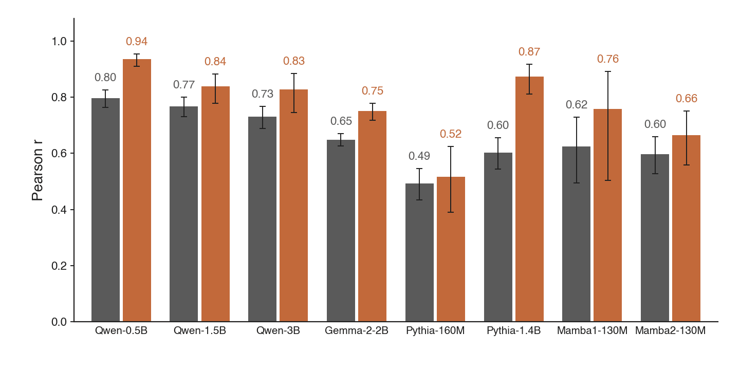
At
Same Idea, Different Tool
If the breakdown really comes from local loss geometry (and not from which method you used to find the direction), then a different first-order interpretability tool should show related failures when the local-linear approximation breaks.
Attribution patching is one such tool, popular as an alternative to direct intervention. Instead of running the full counterfactual activation intervention and measuring the resulting change, you approximate the effect using only the first-order term (the gradient, which indicates how the output changes with small parameter adjustments). This first-order term underpins the method. The method, therefore, assumes higher-order corrections remain small. My proposed formula gives a diagnostic on where the assumption breaks.
Across three model families, on every combination of model and layer where I had a clean enough signal to estimate, attribution patching at
This represents the same off-linear correction encountered with the same tool and equivalent limitations.
The result that didn’t go my way
I want to be honest about one area where the framework fell short when applied as a prescription.
The benchmark is SAEBench-Unlearning. Its task is to make a language model forget specific dangerous knowledge without reducing its general capabilities. The standard method pushes along ten “forget” directions with fixed strength
The standard recipe at
To the person who picked
Regardless, here is what the formula still says. The working multiplier (
Saying “
Where it does win
A second go. This time, I use the formula to describe what’s happening rather than to choose the push strength up front. This is a very clean descriptive result against an aggressive push.
The task is to steer a chat model’s personality (Chen et al., 2025, refer to this as “persona vectors”). These traits: evil, sycophancy, and hallucination. Fifteen prompts per trait. An external model as a judge (Anthropic’s Sonnet 4.6) decides per prompt which response is better on both effect size and coherence. The adaptive
Swapping to a smaller external judge (Mistral-7B-Instruct-v0.3) drops the count to 21/45. Let the model self-judge (Qwen2.5-7B Instruct); it's 29/45. The ranking across all three judges is the same. The absolute count is judge-sensitive, as expected.
What I’d like you to take away from this
One extra column in every steering paper's main table:
The reading rule is also one line. If your push is inside
What I’m still confused about.
Well, a lot of things. I’m 21, so I’m still confused about mortgages, health insurance, and what "carbon copy" in emails means. But for the purpose of this, my confusion is slightly more technical.
The fit that uses all three geometric quantities (not just the gradient
I excluded RWKV-7 (another non-transformer architecture) from the model table. The first-order computation works fine. The second-order computation on this particular architecture yields curvature and third-derivative estimates that are roughly 1000x larger than expected. I think this stems from how the architecture's kernel is made, and that a custom gradient would fix it. I have not tried this.
Some methods for finding directions land inside the safe range much more often than others. The formula tells you which ones do, but not why. I think this is an interesting open question.
Finally, I argue that the safe-push budget should scale in a particular way with the “sharpness” of the model’s output distribution. The data is consistent with that scaling direction, but I haven’t measured the scaling directly. One more state-space model, a matched protocol, should help support this argument.
Connections to other work
Five concurrent threads ask related questions from several angles.
Some people are bounding steering effects by the magnitude of the push vector itself (Hao 2025). My formula uses the geometry of the direction, which is where the divergence of the same two magnitudes occurs. Other people are dynamically setting the budget during steering itself (Muhamed 2025; dynamic SAE gating during unlearning). That dynamic choice fixes a budget that my formula makes explicit. Another is predicting which steering directions will succeed in the first place (Billa 2026). Direct comparison welcome. The same diagnostic shape appears in vision models (Flovik 2025; class-suppression thresholds for image classifiers). One paper converts activation steering into permanent edits to the model's weights (Sun et al., 2026; Steer2Edit).
The underlying machinery is much older. The optimization literature has been using trust-region local Taylor coefficients since before I was born (the 90s). The adversarial-robustness literature has been growing, with closed-form per-input certified radii since 2019 (randomized smoothing, PixelDP). The shape is largely the same: a closed-form per-input radius tied to a measured geometric quantity. This work is that shape, applied to activation-space editing.
Links
Code and proofs at: github.com/jackyoung27/alphasafe.