TL;DR:

We introduce the R-lens: a drop-in replacement for J-lens that produces clearer readouts on earlier layers. R-Lens is identical to J-Lens, except that we make minor and low-overhead changes to the backwards pass, following layerwise-relevance propagation, allowing us to reduce the propagation of errors. This method allows us to surface important intermediate variables more consistently and more saliently, reduce the frequency of semantically-irrelevant readouts, and even detect relevant concepts that J-lens misses entirely. We open-source our R-lenses and accompanying J-lenses here.

Introduction

Motivation

The J-lens is a powerful tool for surfacing intermediate variables in the workspace layers of a model, but we find readouts in early layers to often be noisy and largely uninterpretable. Plausibly, either J-lens is degenerate at these depths and fails to resolve content that is in fact present, or the early residual stream genuinely carries no linearly accessible, causally relevant verbalizable content.

We suspect that this is a structural issue with J-lens. J-lens is fit by backpropagating from the final-layer residual stream down to the residual stream at the readout layer. Errors are likely to accumulate over the course of layers, suggesting it may be less accurate at early layers. In this post, we ask whether we can improve on J-lens to minimize such errors and achieve cleaner, causally relevant readouts at early layers.

What is RelP and how do we apply it?

We take inspiration from Relevance Patching (RelP), a method for efficiently approximating attribution patching, a gradient based approximation to activation patching. It keeps the structure of attribution patching, which takes the dot product of an activation difference against a backward-pass, but swaps the local gradient for a propagation coefficient derived from the XAI technique of Layer-wise Relevance Propagation (LRP). LRP adds several stop gradients to the backward pass, e.g to the variance term in LayerNorm, designed to reduce the accumulation of errors/high curvature gradient terms. As this is just adding stop gradients, the cost is negligible.

We therefore use LRP as a drop-in replacement inside J-lens. We fit the R-lens exactly as before but with LRP rules installed in the backward pass, so what gets transported and averaged is a relevance coefficient rather than a raw gradient.

Contributions

• R-lens shows a substantial quantitative advantage over J-lens that increases as models scale, measured across a variety of evaluation categories.
• R-lens produces qualitatively different readouts at earlier layers, significantly reducing the amount of incoherent tokens compared to J-lens.
• Through ablation studies, we show that R-lens directions for intermediate variables are more causally important than J-lens directions.
• R-lens can sometimes capture concepts that J-lens never does, especially if these concepts appear exclusively in early layers (however, because concepts typically appear in later layers as well, R-lens is primarily a tool for more faithfully tracking computation over layers).

Background

J-lens

The Jacobian lens characterizes an activation by its first-order causal effect on the model's outputs, averaged over contexts and token positions. Concretely, it replaces every layer downstream of the readout point with a single linear map, followed by the model's own unembedding, producing a ranked list of vocabulary tokens for that activation.

LRP

LRP assigns a relevance score to each component and propagates it backward through the model, redistributing relevance from a layer's outputs to its inputs according to rules specific to each component type. LRP preserves ‘total relevance’ from one layer to the next and constructs specialized rules to patch relevance in places where ordinary gradients would break that conservation. Notably, LRP just adds stop gradients, so it is cheap and doesn't change the output of the forward pass.

In particular, we make use of three LRP rules:

• LN-rule: treat the normalization denominator as constant, making the norm linear and preventing relevance collapse.
• Identity-rule: detach the nonlinear factor of GELU/SiLU, so the activation's backward pass becomes a per-element linear map. i.e. replace with stop_grad(GELU)
• Half-rule: split relevance evenly across a multiplicative gate's two branches instead of double-counting through the product.

Methods: the R-Lens

Dense models

• What we modify
  • LN-rule on the residual-stream RMSNorms: replace the forward with a copy that detached the normalization factor
  • Identity rule + half-rule on the gated MLP: The identity-rule makes SiLU backward a per-element linear map (gradient is just sigmoid(z) instead of the full SiLU derivative), and the half-rule splits relevance evenly between the gate path and the up path instead of double-counting through the bilinear product
• What we do not modify:
  • All linear layers (the LRP 0-rule produces the same thing as autograd’s ordinary gradient)
  • Attention
  • q/k norms

MoE models

• We use a similar setup to dense models, with a few modifications to account for the architectural differences:
  • We extend the LRP rules to all routed experts (i.e. we treat all experts as if they were normal MLP layers)
  • We freeze the expert routing weights (+softmax/sigmoid scoring, router logits, and gate projection)
  • Some models have a shared expert, which is always on. We multiply the shared expert’s output by a constant and sweep over a few values of the constant, which amplifies the shared expert’s importance
  • Note: DeepSeek-v4-flash’s residual stream uses manifold-constrained hyper-connections (mHC), which means that the state carried between sublayers is a matrix .
    • For this model, we additionally freeze the mHC residual-mixing coefficients

Results

Quantitative comparisons

Evals

Our evals are similar in content to those described in Appendix A.6 of the J-lens paper. We probe on the bolded token position:

• Multihop: 2-hop factual questions
  • Example:
    • Prompt: “the color of the planet fourth from the Sun is”
    • Intermediate: “Mars”
• Multilingual: model using English representations given a non-English prompt
  • Example:
    • Prompt: “lo opuesto de ‘grande’ es” (“the opposite of ‘big’ is”)
    • Intermediate: “small”
• Association: a short passage that evokes an unnamed concept
  • Example:
    • Prompt: “She couldn't buy groceries anymore without strangers whispering, pointing, and holding up their phones.”
    • Intermediate: “fame”
• Typo: a passage with a common misspelled word
  • Example:
    • Prompt: “We made a reservation at our favorite resturant"
    • Intermediate: “restaurant”
• Poetry: the first half of a rhyming couplet
  • Example:
    • Prompt: “A rhyming couplet:\nA wagging tail came bounding through the fog,\n”
    • Intermediate: “dog”

For each model we filtered for the questions the model was capable of answering correctly (for multihop and multilingual).

Metrics

• Mean pass@10 over layers and categories (i.e. in layer x, does the intermediate appear in the top 10 J-lens readout at the target position)
• Pass@10 per layer and per category

Results

• R-lens shows a substantial quantitative advantage over J-lens as models scale
  • There is no R-lens advantage for both the smallest dense and MoE models we tested. But the R-lens for every other model shows an improvement over J-lens, for both pass@10 averaged over the first half of layers and averaged over all layers. This advantage increases with model size, with the R-lens for DeepSeek-V4-Flash (a 284B-parameter/13B-active MoE model) showing the largest advantage.
  • Eval performance across layers and for individual eval categories shown below for each model

Qualitative comparisons

Layer at which the target concept first appears

• The R-lens often surfaces important intermediate concepts at earlier layers than the J-lens
• Typo prompt example:
  • On the misspelled word “aganst”, R-lens surfaces the correctly-spelled “against” at rank 1 at layer 4, while J-lens never surfaces “against” on the token position where the typo occurs

• Multihop prompt example: “The capital of the country where sushi originated is”
  • On the token “sushi”, R-lens surfaces the intermediate “Japan” at layer 2, while J-lens does not surface it until layer 14

• Basic readout prompt example: “The athlete Michael Jordan plays the sport of”
  • On the token “Jordan”, R-lens surfaces the token “basketball” at layer 4, while J-lens surfaces it at layer 20

R-lens is generally more coherent in early layers than J-lens

• In early layers, J-lens tends to contain what we refer to as “trash tokens”: tokens that are seemingly non-semantic, incoherent, or unrelated to the prompt
  • E.g. “锁定” ("locking"), “尷” (half of "awkward"), “＊＊＊＊＊＊＊＊”, “ ...\n\n”, “......”, “euw”, “tav”, “zinho”, etc.
• One conclusion you might draw from this is that J-Lens is working as intended, and early layers do not contain the types of “verbalizable representations” that define workspace content, so there is in effect nothing for J-lens to surface. However, the fact that R-Lens works shows this is clearly false.
• We can quantify this and see that R-lens seems to contain drastically fewer trash tokens in the early layers.
  • Even if they're not super informative, they show clear structure, e.g. representing the current token or similar tokens
    • E.g. for the prompt below, after “color”, we see “颜色的” (“of color” in Chinese); after “fourth”, we see “fifth”
  • We even see examples of “interpretative meta-tokens” coming up on very early layers
    • E.g. for the prompt below, the token “是什么呢” (“what is this?”) pops up as early as L6 when the model is trying to do the multihop computation

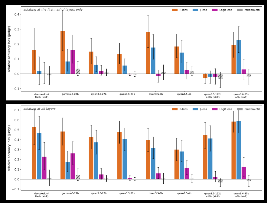
We perform ablations to determine the causal importance of R-lens and J-lens directions

Setup: on 30 questions from the multihop eval set, we ablate the projection of the R-lens, J-lens, and logit lens directions for the intermediate token from the activations on the penultimate token position of the prompt.

• • We test ablating only on the first half of layers (to test saliency of early representations for each method) and ablating on all layers
  • We test the relative accuracy loss (judged with a GPT 5.4 nano autorater): we sample each prompt 8 times before and after ablating, and measure the reduction in accuracy across all 30 prompts
• Results:
  • On nearly all models (with the exception of the two smaller MoEs on the first half of layers), ablating the R-lens directions for the intermediates results in a much larger decrease in accuracy than ablating J-lens or logit lens directions.
  • This suggests that the R-lens directions for intermediates are more causally important for determining the answer, especially on the largest model, Deepseek-V4-Flash.

R-lens captures early-layer concepts that J-lens never surfaces:

• We show above that R-lens is often able to read out concepts at earlier layers than J-lens. Typically, these concepts show up in later layers and are eventually read by J-Lens. This means R-Lens is a valuable tool for tracking computation over layers, but less so for just detecting the presence of concepts.
• However, in certain cases R-lens can surface concepts that appear exclusively in earlier layers, which J-lens entirely misses
• Example: on the token “Verona”, R-lens surfaces “Italy” at rank 1 around layer 5, while it has rank >1000 with J-lens

• Example: in a prompt briefly mentioning Albert Einstein, the token “ physicists” is surfaced in the top 10 by R-lens around layers 6-17 but not by J-lens

We train probes to upper bound the earliest layer we can expect lens readouts

• Setup:
  • We train linear probes to distinguish between 10 concepts within a category (e.g. for athletes, we train a linear classifier on 10 famous athletes)
  • On a simple factual recall question (e.g. “The athlete Michael Jordan plays the sport of”), we find the earliest layer where these probes get 0.99-1.00 accuracy
    • These layers represent a crude “upper bound” on how early we can expect lens readouts to identify concepts. We don't take it too seriously (and in the case of landmarks, R-Lens beats it)
• Results:
  • We find that R-lens consistently appears at earlier layers than J-lens, getting significantly closer to the probe-defined upper bound.

CKA Analysis

We found R-lens to be more different than J-lens in early layers and the R-space CKA to show roughly 2-3 distinct bands as opposed to J-space CKA’s 4-5 for Qwen-3.6-27b.

Appendix

Do MLP layers preferentially amplify RelP lens directions?

We measure the MLP gain (how strongly the information encoded by a direction v is amplified by the next MLP block) of directions from J-lens, R-lens, and logit lens compared to those of a standard MLP neuron. This is similar to the experiment from Figure 32 of the J-lens paper. We find that on Qwen3.6-27B, J-lens and R-lens directions are similarly amplified across layers, and these are significantly more amplified than the MLP neuron in later workspace layers.

Quantitative eval results for other models