In want of a quantifiable way to decide what counts as a frontier AI model, compute thresholds have emerged as the standard for AI policy: California’s SB 53 uses 10^26 floating-point operations (FLOPs) in the training run as the threshold for what counts as a frontier model and the EU AI Actapplies the same categorization at 10^25. Proposals for international AI agreements (example 1, example 2, example 3) extend the use of training FLOPs to determine part or all of the threshold for what counts as a frontier model under the agreement. Current AI laws have no way of actually verifying AI companies’ claims about the number of FLOPs used in training and instead just rely on self-reports, but an international AI agreement can’t assume compliance from each involved party. As such, we’d like to verify the number of FLOPs used in LLM training runs through side-channel GPU readings. This allows AI developers’ code and data to remain hidden from the verifiers of the AI agreement, but allow verification of training FLOPs even under conditions where the model training might be adversarially changed to circumvent them. My work builds a Minimum Viable Product (MVP) for how this verification could work on an Nvidia Jetson Orin Nano.
Related Work
EpochAIhas done work on estimating the number of training FLOPs using (1) insider knowledge about the model architecture and (2) open-source reports of the number of accelerators, amount of time used in training runs, and expected utilization rate. My estimator extends their method (2) to include power-monitoring and real-time data on utilization.
Chaudhuri et al.demonstrate how thermal and power side-channels, along with assumptions about model architecture, can be used to extract information about transformer model weights during a training run. While an explicit goal of AI treaty verification is to NOT expose model secrets to the verifiers, this shows that extracting information about transformer training runs through side-channels is possible.[1]
Recently, Rahman and Tajdarishowed how GPU system-level readings could be used to classify AI workloads as training vs. inference.
Methodology
Hardware and Observable Signals
All experiments are run on an Nvidia Jetson Orin Nano 8 GB developer kit. This is essentially Nvidia’s version of the Raspberry Pi, a single-board computer used for small-scale experiments and edge computing, but with an Ampere GPU. To estimate FLOPs, we run a sample LLM training script on the Nano and then observe the following signals:
Power (W): The Nano comes with an onboard INA3221 sensor which measures the power consumed by the board in three channels: VDD_IN - the total input power to the board, VDD_CPU_GPU_CV - the power consumed by the shared CPU/GPU/CV Accelerator rail, and VDD_SOC - the power draw of the memory subsystem. For the estimator, I use VDD_CPU_GPU_CV which means we have no way of separating CPU vs GPU power draw, however, we can expect GPU power to dominate the reading.
Memory Bandwidth Utilization (%): Actmonis a hardware activity monitor which reports whether the External Memory Controller (EMC) is active. The EMC is the hardware block which manages the transfer of data between the GPU and DRAM. What this reading does not tell us is how much data is transferred, just whether or not the controller is active. Still, a higher EMC utilization suggests there is a lot of data that needs to be transferred between the GPU from DRAM which can be indicative of a training run happening.
Constructing Sample Workloads
The Nano is not a device that is suitable for running an actual LLM training workload, so instead I use a script that mimics the behavior of a real workload. It initializes a transformer and then runs a training loop for a preset number of steps on randomly generated tokens and can be configured with a range of hyperparameter settings explained below.
Model Width (d_model): the size of the vector representing each token as it flows through the model. A larger model width will quadratically increase the size of matrix multiplications that happen during training.
Depth (n_layers): how many identical transformer blocks are there in total? The total number of operations in the training run will scale linearly with the number of blocks.
Attention heads (n_heads): How many parallel attention operations are used on the input token vector? This doesn’t impact the total number of operations.
Feed-forward width (d_ff): the hidden dimension of the two-layer Multi-Layer Perceptron (MLP) in each transformer block
Sequence length (seq_len): how many tokens are processed together in parallel? This increases the computation done by the MLP linearly and the attention heads quadratically.
Batch size: how many sequences of tokens are processed in a single step? In a real LLM training setup, changing this would not be expected to have a big impact on FLOPs because although more sequences are processed in parallel, there is typically only a fixed number of tokens for the training run to get through. However, in this experimental setup, the tokens are made up as the training run goes for a fixed number of steps, so we should expect FLOPs to increase linearly with batch size.
Optimizer (Adam vs. SGD): The algorithm used for updating model weights during training. The size of these operations should be dwarfed by the much larger matrix multiplications.
Numeric Precision (FP32/TF32/FP16/BF16): What precision to represent every number in during the training run? Changing this shouldn’t affect the ground truth FLOPs, but might confuse the estimator since an FP16 operation will be less intensive than an FP32 operation. For keeping this experiment simple, I am only testing on FP32, but future work will involve expanding this to work across multiple types of precision.
While the sample training run script can simulate a workload with any value of hyperparameters, we only care about the FLOP estimator being accurate on workloads which emulate a realistic training run that an AI developer might actually do. In practice, we’d expect an AI developer to want to fully utilize their GPUs as best as they can, so I define “frontier” sample training runs as ones in which the GPU is active at least 80% of the time, as reported by polling tegrastats, a profiling tool on the Jetson . Note, this is different from the EMC bandwidth utilization percentage which is measuring how often the memory controller is running. Since I was unsure which hyperparameters to use to be above the 80% threshold, I ran the script under a bunch of hyperparameter configurations and only kept the ones which utilized the GPU above the 80% threshold on average.
Ground Truth Computation
We can get the ground truth for the number of FLOPs by looking at the shapes of tensors involved in the training algorithm. For example, multiplying an (m×k) matrix by a (k×n) matrix requires m·n·k multiplications and roughly as many additions, so we could count this as 2·m·k·n FLOPs towards the ground truth, regardless of how the hardware executes this at the lowest level. To get the ground truth FLOPs for the various sample training runs in my experiments, I used PyTorch’s FlopCounterMode library. This library hooks onto PyTorch to intercept every tensor shape as it is used in low-level operations during the training run and dynamically compute the algorithmic FLOPs as the program executes.
The FLOP Estimator
The estimator’s algorithm is shown below in equation (1).
I explain terms below, but first, let me motivate on a high level what this equation is doing. In the simplest case, we would like to just figure out how much energy the GPU is using, calibrate our Energy_Per_TFLOP parameter based on a bunch of workloads with known total FLOP counts, and then predict on held-out examples based on this GPU energy reading. The issue, though, is that we can only get total energy consumption on the Nano and don’t have any knowledge of how much of that the GPU is directly responsible for. So, this is where the additional terms, TB_moved and P_overhead, come in to represent the energy consumed by the memory bus and non-GPU-related activity (fans, disk, etc.), respectively. The result is that after calibrating all parameters, the terms in the numerator should approximate the energy consumption the GPU is directly responsible for.
E_net (J): This is the energy derived from power measured by the INA3221 sensor minus the idle baseline power measured during the calibration phase, integrated over time
E_PER_TB (J/TB): The energy cost of moving one terabyte of data between DRAM and the GPU. It is a constant set during the calibration phase.
TB_moved: The total number of terabytes transferred between DRAM and the GPU during the workload. This is measured actively during estimation by monitoring the activity of the EMC.
t (s): The total duration of the workload in seconds as determined in the monitoring daemon
E_PER_TFLOP (J/TFLOP): The total energy cost of one TFLOP of GPU compute. In practice, this is whatever energy is left over after accounting for the idle baseline, CPU workload overhead, and memory bus overhead. During estimation, this is a constant that is set during the calibration phase.
P_Overhead (W): This is the fixed overhead power that we would expect from running any job. The hope is that this will account for the portion of power draw spent by parts of the Jetson other than the GPU, like the CPU and the fan.
Detecting Workloads
In order to estimate the number of FLOPs in a workload, the estimator needs to know when a new workload has started and when it ends. To do this, the estimator is deployed in a daemon which polls for GPU utilization every 1.5 seconds; equation (1) is computed at each interval based on the samples from the power sensor and EMC. A new workload starts when GPU utilization is above 5% for two consecutive polls and ends when 3 consecutive polls are below 5%. At the end of a detected workload, the daemon accumulates the power and bandwidth utilization logged over the course of the session along with the total time elapsed and outputs a total FLOP estimate for the workload which is then compared against the ground truth given by FlopCounterMode to determine accuracy.
Figure 1
Methodology overview: calibration phase is run first, followed by using the calibrated constants during the deployment phase
Results
Calibration Phase
Before the FLOP estimator daemon can be run on any workloads, we must first calibrate the estimation parameters. Re-running this estimator on different hardware would require re-doing this calibration phase and getting different values for these terms.
Idle Power: For this, we just need to measure the power of the Nano while it is sitting idle. I do this with a script that just does nothing for 90 seconds except poll the INA3221 at 2 Hz and take the median at the end. This came out to 642 mW, so during estimation, I subtract this from the INA3221 reading to get E_net. For reference, the Nano, set at its default power setting, is allowed a maximum power consumption of 25 W.
Power Overhead: This is likely the most loosely fitted calibrated parameter. We would want it to capture the overhead energy cost of non-GPU activity while a GPU workload is running, however, there isn’t really a way to run a GPU workload that is active, but not doing anything. This is calibrated by fitting the parameter to a set of calibration workloads with known FLOP ground truths.
Energy per TB: Calibrated on validation workloads by fitting to the constant value that results in the estimator having the lowest mean squared error.
EMC Scale Factor: As mentioned in the methodology, we can only read when the EMC is active, not how many bytes have been transferred. However, we know that the Nano’s maximum memory bandwidth is 102 GB/s, so we can run a script to load a known amount of bytes onto the GPU from memory, read the EMC data from the system, and calibrate a scaling factor that can approximate the number of bytes being transferred.
Energy Per TFLOP: As in Power Overhead, calibrated on calibration workloads with known FLOP counts.
Estimator Accuracy
After we calibrate the estimator, we can run it on held-out workloads to get its accuracy as a percentage error compared to the ground truth FLOP count given by FlopCounterMode. Getting pinpoint accuracy on the number of FLOPs used in sample training runs was never going to be possible, but my hope was that the estimator could at least be less than 10% off just as an arbitrary threshold for good-enough accuracy. As a validation check I ran a sample workload for ~10 minutes and collected the power (Figure 2) and bandwidth utilization (Figure 3) traces every 0.5s.
Figure 2
Figure 3
To calibrate and evaluate the estimator, I run a suite of 26 sample training-run configurations sweeping the hyperparameters described in the methodology, back-to-back in a single session against one shared idle baseline, with each workload training for 900 - 4,800 steps and reporting its ground-truth FLOP count via FlopCounterMode. Of these, 21 cleared the 80% frontier-utilization gate to be used for calibration and evaluation. On these 21 “frontier” workloads, I randomly split them into 14 calibration (only used for calibrating the estimator parameters) and 7 testing workloads (only used for evaluation; held-out during calibration). This is repeated 200 times, so that for any given workload, the estimator is calibrated with differing training workloads and then evaluated on that workload ~67 times. Figure 4 shows the difference between estimated tera-FLOPs (TFLOPs) and the ground truth for each of the 21 workloads, with the minimum and maximum predicted TFLOPs for that workload over the course of the 200 runs.
Figure 4
All of the 21 different points on Figure 4 represent applying the estimator to one of the sample training workloads, which each have different hyperparameter configurations. Figure 5 below shows how the estimator’s error (whether it over- or underestimated) changes under different hyperparameters for the sample workload script. I run each of the 21 workloads 3 times, and then record the estimator’s error along with the hyperparameter configurations. It should be noted that we cannot infer causality from these results, as changes in one hyperparameter value are often confounded by a change to another value that is needed to keep the workload above the “frontier” utilization threshold.
Figure 5
As an ablation, I also test a 2-parameter version of the estimator that no longer reads sensor input from the EMC, and only looks at power from the INA3221 power sensor. Equation 2 shows the calculation performed by this version of the estimator which just drops the energy-per-TB-moved term. Figure 6 shows the results of fitting this estimator on 200 train/test splits (the same as for figure 4) and comparing the estimated TFLOPs to the ground truth.
Figure 6
In summary, the results show that across 200 random train/test splits, the estimator's held-out predictions had a mean absolute error of 4.5% (σ = 3.8%) with negligible average bias (mean signed error −0.4%), though 59% of splits contained at least one workload exceeding the 10% target error.
Next Steps
The Jetson Orin Nano is a useful device for doing easy, non-compute-intensive experiments, but stress-testing FLOP estimation on real AI data center hardware would be more fitting to how this could get used in a real verification situation. As a step toward that more realistic setting, I will replicate this on a dual-GPU V100 SXM2 node that I have physical access to. From here, I’d like to also incorporate the size of data transfer between GPUs during training as an additional input to the FLOP estimation model.
In addition to not being run on real AI data center hardware, another limitation of this initial, proof-of-concept experiment is the lack of adversarial testing. In a verification regime, not only do we need FLOP estimation to avoid having to rely on possibly-false self-reports, but we also must assume adversarial behavior on behalf of the AI model developers. Currently, my experiments only test if we can estimate FLOPs accurately on benign LLM training workloads, not workloads which have been adversarially designed to fool the estimator into outputting a lower FLOP count than what actually happened.
Other next steps which I think need to be done, but I am not currently prioritizing:
Reframing FLOP estimation accuracy as false positive/negative rate for a classification of a training load as above/below a certain threshold. This would allow us to, say, tolerate a higher rate of false positives than false negatives.
Security challenges: we both want to make sure verifiers don’t get too much access that they can uncover secrets about the training run and we want to make sure model developers can’t directly hack the estimator.
I expect FLOP estimation would be best suited as another layer of swiss cheese than as the end-all be-all threshold for what is an allowed vs disallowed training run. Future work should include incorporating it into other forms of verification, like verifying training vs inference, monitoring cluster ingress/egress, and tamper-detection.
I am interested in getting feedback on any interesting next steps I am missing and on this project in general.
Thanks to Shahin Tajik, Justin Chen, and Madeleine Hoffman for their help reviewing an earlier version of this report.
This work is supported by the University of Chicago Existential Risk Laboratory.
For the sake of my project, I would just like to work on the verification aspects and leave improving the security for later. It seems bad that there is research showing you can extract model weights using side-channels as this would undermine the assumption that AI developers’ code would remain secret. In practice, though, I think this would be a much more difficult task than just getting the side-channel measurements you’d need for estimating FLOPs.
This is a research summary for an ongoing project I am working on as part of the UChicago Existential Risk Laboratory Summer Research Fellowship. I would really appreciate any feedback.
Introduction
Motivation
In want of a quantifiable way to decide what counts as a frontier AI model, compute thresholds have emerged as the standard for AI policy: California’s SB 53 uses 10^26 floating-point operations (FLOPs) in the training run as the threshold for what counts as a frontier model and the EU AI Act applies the same categorization at 10^25. Proposals for international AI agreements (example 1, example 2, example 3) extend the use of training FLOPs to determine part or all of the threshold for what counts as a frontier model under the agreement. Current AI laws have no way of actually verifying AI companies’ claims about the number of FLOPs used in training and instead just rely on self-reports, but an international AI agreement can’t assume compliance from each involved party. As such, we’d like to verify the number of FLOPs used in LLM training runs through side-channel GPU readings. This allows AI developers’ code and data to remain hidden from the verifiers of the AI agreement, but allow verification of training FLOPs even under conditions where the model training might be adversarially changed to circumvent them. My work builds a Minimum Viable Product (MVP) for how this verification could work on an Nvidia Jetson Orin Nano.
Related Work
EpochAI has done work on estimating the number of training FLOPs using (1) insider knowledge about the model architecture and (2) open-source reports of the number of accelerators, amount of time used in training runs, and expected utilization rate. My estimator extends their method (2) to include power-monitoring and real-time data on utilization.
Chaudhuri et al. demonstrate how thermal and power side-channels, along with assumptions about model architecture, can be used to extract information about transformer model weights during a training run. While an explicit goal of AI treaty verification is to NOT expose model secrets to the verifiers, this shows that extracting information about transformer training runs through side-channels is possible.[1]
Recently, Rahman and Tajdari showed how GPU system-level readings could be used to classify AI workloads as training vs. inference.
Methodology
Hardware and Observable Signals
All experiments are run on an Nvidia Jetson Orin Nano 8 GB developer kit. This is essentially Nvidia’s version of the Raspberry Pi, a single-board computer used for small-scale experiments and edge computing, but with an Ampere GPU. To estimate FLOPs, we run a sample LLM training script on the Nano and then observe the following signals:
Constructing Sample Workloads
The Nano is not a device that is suitable for running an actual LLM training workload, so instead I use a script that mimics the behavior of a real workload. It initializes a transformer and then runs a training loop for a preset number of steps on randomly generated tokens and can be configured with a range of hyperparameter settings explained below.
While the sample training run script can simulate a workload with any value of hyperparameters, we only care about the FLOP estimator being accurate on workloads which emulate a realistic training run that an AI developer might actually do. In practice, we’d expect an AI developer to want to fully utilize their GPUs as best as they can, so I define “frontier” sample training runs as ones in which the GPU is active at least 80% of the time, as reported by polling tegrastats, a profiling tool on the Jetson . Note, this is different from the EMC bandwidth utilization percentage which is measuring how often the memory controller is running. Since I was unsure which hyperparameters to use to be above the 80% threshold, I ran the script under a bunch of hyperparameter configurations and only kept the ones which utilized the GPU above the 80% threshold on average.
Ground Truth Computation
We can get the ground truth for the number of FLOPs by looking at the shapes of tensors involved in the training algorithm. For example, multiplying an (m×k) matrix by a (k×n) matrix requires m·n·k multiplications and roughly as many additions, so we could count this as 2·m·k·n FLOPs towards the ground truth, regardless of how the hardware executes this at the lowest level. To get the ground truth FLOPs for the various sample training runs in my experiments, I used PyTorch’s FlopCounterMode library. This library hooks onto PyTorch to intercept every tensor shape as it is used in low-level operations during the training run and dynamically compute the algorithmic FLOPs as the program executes.
The FLOP Estimator
The estimator’s algorithm is shown below in equation (1).
I explain terms below, but first, let me motivate on a high level what this equation is doing. In the simplest case, we would like to just figure out how much energy the GPU is using, calibrate our Energy_Per_TFLOP parameter based on a bunch of workloads with known total FLOP counts, and then predict on held-out examples based on this GPU energy reading. The issue, though, is that we can only get total energy consumption on the Nano and don’t have any knowledge of how much of that the GPU is directly responsible for. So, this is where the additional terms, TB_moved and P_overhead, come in to represent the energy consumed by the memory bus and non-GPU-related activity (fans, disk, etc.), respectively. The result is that after calibrating all parameters, the terms in the numerator should approximate the energy consumption the GPU is directly responsible for.
Detecting Workloads
In order to estimate the number of FLOPs in a workload, the estimator needs to know when a new workload has started and when it ends. To do this, the estimator is deployed in a daemon which polls for GPU utilization every 1.5 seconds; equation (1) is computed at each interval based on the samples from the power sensor and EMC. A new workload starts when GPU utilization is above 5% for two consecutive polls and ends when 3 consecutive polls are below 5%. At the end of a detected workload, the daemon accumulates the power and bandwidth utilization logged over the course of the session along with the total time elapsed and outputs a total FLOP estimate for the workload which is then compared against the ground truth given by FlopCounterMode to determine accuracy.
Figure 1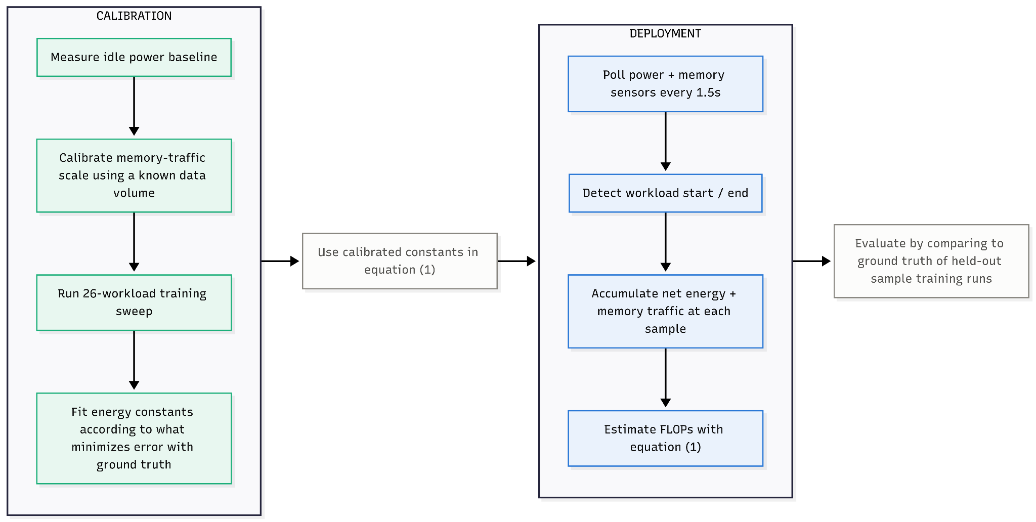
Methodology overview: calibration phase is run first, followed by using the calibrated constants during the deployment phase
Results
Calibration Phase
Before the FLOP estimator daemon can be run on any workloads, we must first calibrate the estimation parameters. Re-running this estimator on different hardware would require re-doing this calibration phase and getting different values for these terms.
Estimator Accuracy
After we calibrate the estimator, we can run it on held-out workloads to get its accuracy as a percentage error compared to the ground truth FLOP count given by FlopCounterMode. Getting pinpoint accuracy on the number of FLOPs used in sample training runs was never going to be possible, but my hope was that the estimator could at least be less than 10% off just as an arbitrary threshold for good-enough accuracy. As a validation check I ran a sample workload for ~10 minutes and collected the power (Figure 2) and bandwidth utilization (Figure 3) traces every 0.5s.
Figure 2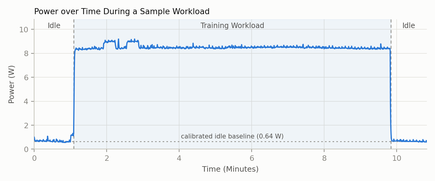
Figure 3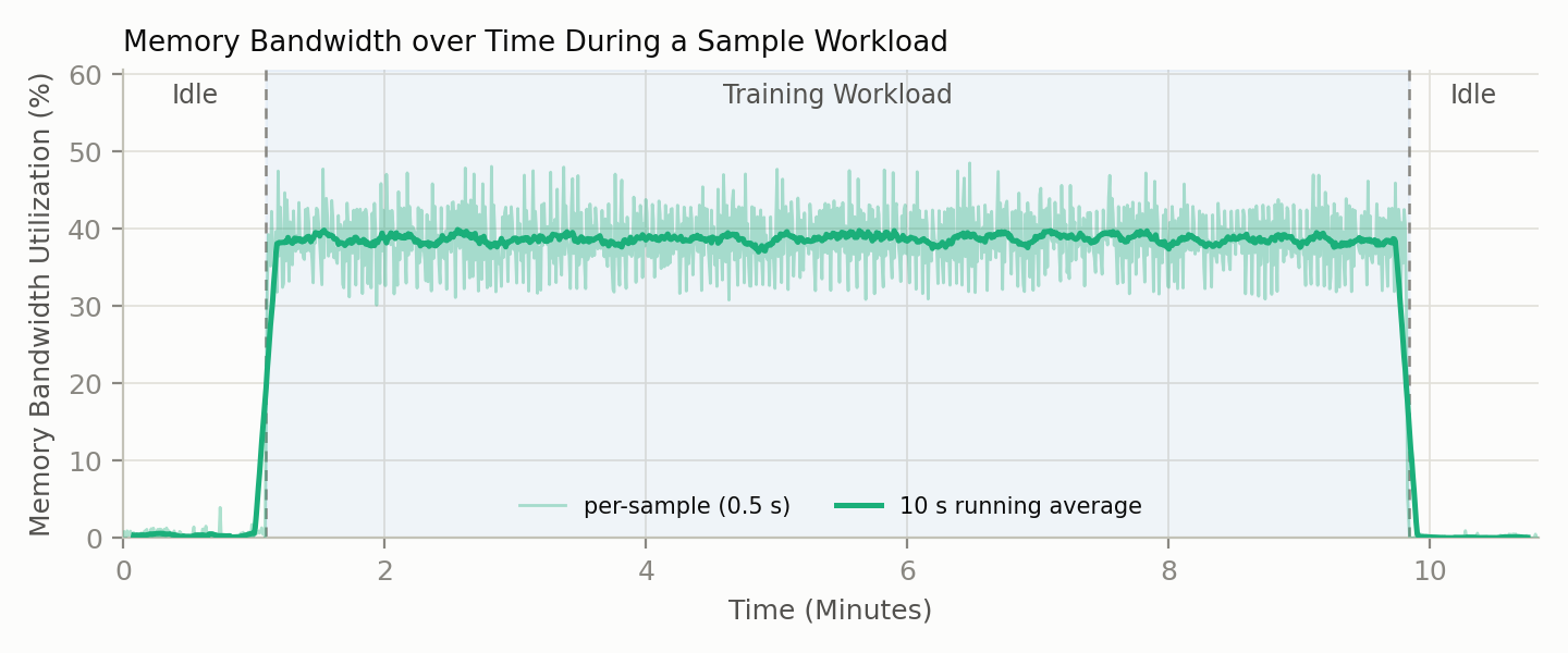
To calibrate and evaluate the estimator, I run a suite of 26 sample training-run configurations sweeping the hyperparameters described in the methodology, back-to-back in a single session against one shared idle baseline, with each workload training for 900 - 4,800 steps and reporting its ground-truth FLOP count via FlopCounterMode. Of these, 21 cleared the 80% frontier-utilization gate to be used for calibration and evaluation. On these 21 “frontier” workloads, I randomly split them into 14 calibration (only used for calibrating the estimator parameters) and 7 testing workloads (only used for evaluation; held-out during calibration). This is repeated 200 times, so that for any given workload, the estimator is calibrated with differing training workloads and then evaluated on that workload ~67 times. Figure 4 shows the difference between estimated tera-FLOPs (TFLOPs) and the ground truth for each of the 21 workloads, with the minimum and maximum predicted TFLOPs for that workload over the course of the 200 runs.
Figure 4
All of the 21 different points on Figure 4 represent applying the estimator to one of the sample training workloads, which each have different hyperparameter configurations. Figure 5 below shows how the estimator’s error (whether it over- or underestimated) changes under different hyperparameters for the sample workload script. I run each of the 21 workloads 3 times, and then record the estimator’s error along with the hyperparameter configurations. It should be noted that we cannot infer causality from these results, as changes in one hyperparameter value are often confounded by a change to another value that is needed to keep the workload above the “frontier” utilization threshold.
Figure 5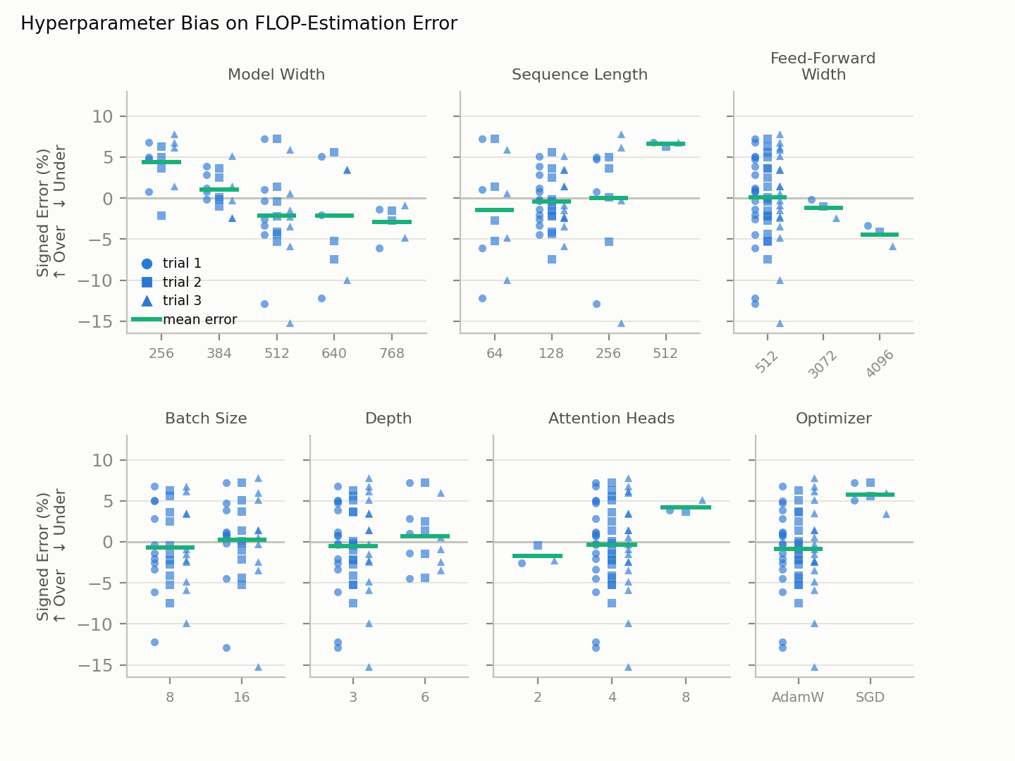
As an ablation, I also test a 2-parameter version of the estimator that no longer reads sensor input from the EMC, and only looks at power from the INA3221 power sensor. Equation 2 shows the calculation performed by this version of the estimator which just drops the energy-per-TB-moved term. Figure 6 shows the results of fitting this estimator on 200 train/test splits (the same as for figure 4) and comparing the estimated TFLOPs to the ground truth.
Figure 6
In summary, the results show that across 200 random train/test splits, the estimator's held-out predictions had a mean absolute error of 4.5% (σ = 3.8%) with negligible average bias (mean signed error −0.4%), though 59% of splits contained at least one workload exceeding the 10% target error.
Next Steps
The Jetson Orin Nano is a useful device for doing easy, non-compute-intensive experiments, but stress-testing FLOP estimation on real AI data center hardware would be more fitting to how this could get used in a real verification situation. As a step toward that more realistic setting, I will replicate this on a dual-GPU V100 SXM2 node that I have physical access to. From here, I’d like to also incorporate the size of data transfer between GPUs during training as an additional input to the FLOP estimation model.
In addition to not being run on real AI data center hardware, another limitation of this initial, proof-of-concept experiment is the lack of adversarial testing. In a verification regime, not only do we need FLOP estimation to avoid having to rely on possibly-false self-reports, but we also must assume adversarial behavior on behalf of the AI model developers. Currently, my experiments only test if we can estimate FLOPs accurately on benign LLM training workloads, not workloads which have been adversarially designed to fool the estimator into outputting a lower FLOP count than what actually happened.
Other next steps which I think need to be done, but I am not currently prioritizing:
I am interested in getting feedback on any interesting next steps I am missing and on this project in general.
Thanks to Shahin Tajik, Justin Chen, and Madeleine Hoffman for their help reviewing an earlier version of this report.
This work is supported by the University of Chicago Existential Risk Laboratory.
For the sake of my project, I would just like to work on the verification aspects and leave improving the security for later. It seems bad that there is research showing you can extract model weights using side-channels as this would undermine the assumption that AI developers’ code would remain secret. In practice, though, I think this would be a much more difficult task than just getting the side-channel measurements you’d need for estimating FLOPs.