An examination of the effect of model size on interpretability
I. Executive summary
This is the third installment of a series of analyses exploring basic AI mechanistic interpretability techniques. While Part 1 and Part 2 in this series are summarized below, a review of those articles will provide the reader with helpful context for the analysis contained herein.
Key findings
The analysis below compares the application of matched-pairs text samples and pretrained residual stream sparse autoencoders (“SAEs”) in conjunction with both GPT-2 Small 124m (used in Parts 1 and 2 of this series) and Gemma 2 9b.
The following analyses showed that specialist features’ strongly focus on syntax over semantics persists in both models
Both models exhibit a 2-tier representational structure wherein specialist features detect syntax while overall representation (not just specialists) demonstrates semantic-based clustering. This representation is denser, and emerges in later layers in Gemma, compared to GPT-2.
In both models, the degree of specialist feature activation affects both the model’s output and its confidence in that output, but this varies widely by model, topic / surface form, and model layer.
Confidence in these findings:
Confidence in analysis methodology: moderate
Confidence in the ability to apply these findings to additional models: moderate
II. Introduction
This analysis constitutes the third installment in a multi-part series documenting, in relatively simple terms, my exploration of key concepts related to machine learning (“ML”) generally and mechanistic interpretability (“MI”) specifically. The intended application of this analysis is to further understanding and management of model behavior with an eye toward opening new use cases for models and reducing societally harmful outputs.
This analysis does not purport to encapsulate demonstrably new findings in the field of MI. It is inspired by, and attempts to replicate at a small scale, pioneering analysis done in the field of MI by Anthropic and others, as cited below. My aspiration is to add to the understanding of, discourse around, and contributions to, this field by a wide range of key stakeholders, regardless of their degree of ML or MI expertise.
III. Methodology and key areas of analysis
Key areas of analysis
Fundamentally, this installment’s analysis seeks to answer the following question: “How does model size affect that model’s representational behavior?”.
More specifically, this Phase 3 analysis tests the hypotheses listed in Figure 1 below. These are the same hypotheses tested in Phase 2 of this series, with the differentiation being:
the use of an additional model (Gemma 2 9b) and
additional avenues of testing H2 and H3, with an eye toward producing more robust and insightful answers to those hypotheses.
Figure 1: Phase 2 + 3 hypotheses
Hypothesis
Question
Predictions
H1: Specialist Specificity
Do specialist features primarily detect syntax (surface form) or semantics (meaning)?
If syntax: different forms → different specialists; low cross-form overlap.
If semantics: same topic → same specialists regardless of form
H2: Representational Geometry
Does the overall SAE representation (all features, not just specialists) cluster by syntax or by semantics?
If syntax: within-form similarity > within-topic similarity.
If semantics: within-topic similarity > cross-topic similarity.
H3: Behavioral Relevance
Does specialist activation predict model behavior (e.g., accuracy on math completions)?
If yes: higher specialist activation → better task performance; activation correlates with correctness.
Methodology
The methodology employed in this analysis uses two open-source models and their associated SAEs: GPT-2 Small, a relatively tractable, 12-layer, 124 million parameter model used in the first two installments of this series and Google’s Gemma 2, a much more modern, 42-layer, 9 billion parameter model. Both models were obtained via TransformerLens and the relevant pretrained residual stream SAEs from Joseph Bloom, Curt Tigges, Anthony Duong, and David Chanin at SAELens. For GPT-2 small, I used SAEs at layers 6, 8, 10, and 11. For Gemma 2, I used SAEs at layers 23, 30, 37, and 41.
For sample text, this analysis used the same 241 matched-pairs text samples used in Phase 2 of this series (688 text samples total). The text samples span 7 distinct categories and each matched pairs set includes three different variations of the same concept, each varying by the approximate use of unique symbology. An abbreviated list of those matched pairs is shown in Figure A of the appendix. Notable exceptions to this approach were as follows:
The “Python” category used two matched surface forms (“code” and “pseudocode”) per matched pair, instead of three.
The “Non-English” category contained matched pairs with the same general (but not identical, due to translation irregularities) phrases expressed in three non-English languages (Spanish, French, and German). Since these samples are not identical versions of the same idea, it tests a slightly different version of the syntax vs. semantics hypothesis: whether the “Non-English” feature identified in Phases 1 and 2 of this series relates to non-English text generally or a specific language specifically.
To test math completions and the effects of ablation, I also employed a set of LLM-generated sample prompts that were provided to the model. The set included 264 total math problems: 24 simple (8 problems × 3 forms), 18 complex (6 × 3), and 222 hard (74 × 3). Since Gemma 2 answered the relatively basic math problems employed in my Phase 2 analysis with 100% accuracy (the opposite of the problem encountered in Phase 2 of this series, wherein GPT-2 was unable to correctly answer any math completions), I added additional, more challenging problems to better target Gemma 2's failure zones, including negative-base exponents, logarithms, modular arithmetic, nested operations, and complex fractions. I produced each problem in three surface forms (symbolic, verbal, prose) to enable form-dependent analysis. To account for various forms of the correct answer potentially provided by the model (e.g. “⅕” vs. “one-fifth” vs. “20%”), I used an LLM (Claude Sonnet 4.6) to judge whether the model’s completion contained any variation of the correct answer I provided alongside the problem and the model’s completion.
Non-math completions and ablation followed a similar testing construction. That problem set included 96 total tasks, with 36 for Non-English and Formal and 24 for Python. Each domain used its own specialist feature, enabling cross-domain comparison of whether the activation ↔ accuracy relationship is true across domains or specific to any particular domain(s). Python tasks span simple assignment through list comprehension; Non-English tasks use common phrases in French, Spanish, and German; Formal tasks range from legal/academic register through casual conversation.
Abbreviated lists of those prompts are provided in Figure B and Figure C of the appendix and the full datasets for these and all matched pairs are available at this project’s colab.
In addition to recording the activation measurements provided by the relevant SAEs, I used the calculations defined in the appendix to develop a more comprehensive view of the model’s internal representation.
IV. Results
Summary of results
H1: Specialist Specificity — Do specialist features detect syntax or semantics?
Verdict: Syntax (both models)
Question
GPT-2 Small
Gemma 2 9B
Do same-topic forms share specialist features? (mean Jaccard)
0.151 — mostly no
0.181 — mostly no
How often do same-topic forms share zero specialists?
6/19 pairs (32%)
7/19 pairs (37%)
How sharply do specialists distinguish their target form? (mean Cohen's d)
5.11 (baseline)
7.22 (more selective)
How widely are the most-active features shared across surface forms?(top-20 overlap)
18.9%
60.3% (far denser representation)
Do the same forms produce sparse activations in both models? (sparsity ρ)
—
0.87 (strongly preserved)
Interpretation: Both models’ specialist features primarily detect syntax, not semantics, as most clearly illustrated via their low Jaccard similarities (0.151 for GPT-2, 0.181 for Gemma). Gemma's specialists show comparable selectivity to GPT-2's across most categories, with notably higher Cohen's d in a few domains driving a moderately higher overall mean (7.2 vs. 5.1). Gemma’s ~40pp higher overall feature population overlap indicates the top 20 active features (not necessarily specialists) are more widely-shared among sample texts, compared to GPT-2. These observations suggest that Gemma and GPT-2 follow roughly similar representational patterns, but Gemma excels in both recognizing unique syntax and developing a broad set of features shared across a wide range of text.
H2: Representational Geometry — Do full activation vectors cluster by topic or form?
Verdict: Semantics (both models)
Question
GPT-2 Small
Gemma 2 9B
Are same-topic texts more similar to each other than to different-topic texts? (cosine similarity)
0.503 vs. 0.137 (yes)
0.825 vs. 0.695 (yes, with denser representation)
Is the topic-based clustering statistically significant? (permutation test)
p < 0.0001 (yes)
p < 0.0001 (yes)
How much variance does topic structure explain in 2D? (PCA)
12.8% (modest)
52.5% (significant)
Do texts cluster more by topic than by surface form? (silhouette gap)
+0.042 (topic)
+0.080 (topic)
At what point in the network does topic clustering emerge?
All layers
Final layer only
Interpretation: Activation vectors cluster by semantics in both Gemma and GPT-2 (p < 0.0001). Since any given token activates more features in Gemma vs. GPT-2, this means Gemma will have more features shared between the text samples. This increased number of overlapping features increases both within- and cross-topic cosine similarities, shrinking the gap between them. However, Gemma’s greater PCA variance and silhouette gap suggests that its smaller cosine similarity gap is an artifact of denser activations, not decreased semantic-based clustering. Finally, this topic-based clustering emerges in GPT-2’s early layers, whereas in Gemma, topic-based clustering emerges only at the final layer.
H3: Behavioral Relevance — Does specialist activation predict model behavior?
Verdict: Yes (varies widely by model, topic + form, and layer)
Question
GPT-2 Small
Gemma 2 9B
Does activation predict accuracy? (binary r, math)
Final layer: 1/3 All layers: 2/12 (no - floor effect)
Final layer: 3/3 All layers: 9/12 (yes)
Does activation predict accuracy? (binary r, non-math)
Does removing a specialist change output? (ablation, math)
4/12 conditions (yes)
(2/12 conditions) (yes)
Does removing a specialist change output? (ablation, non-math)
3/32 conditions (yes)
4/32 (yes)
Interpretation: Specialist feature activation is related to both model output and confidence, but that relationship varies widely by topic + surface form and model layer. At the final layer of each model, there exists limited correlation between specialist activation and model output or confidence and ablation is similarly ineffective. At intermediate layers, however, we see greater linkages between activation and model behavior, particularly in the math and non-English categories.
Interpretation of results
H1: Specialist features are primarily focused on syntax (both models)
The first avenue of analysis focused on the specialist features associated with each model and the degree to which their syntax vs. semantic focus differs. In Phase 2 of this analysis, I observed that GPT-2’s specialists were far more attuned to syntax vs. semantics. This Phase 3 analysis confirmed this behavior with regards to both GPT-2 and Gemma.
Jaccard Similarity
One approach of demonstrating both models’ specialists syntactic focus was via the use of Jaccard similarity applied to the various surface forms within a given topic. If specialist features focused on semantics, one would expect relatively high Jaccard similarities across the surface forms containing the same concept.
Key takeaway: The Phase 2 finding that specialist features are primarily syntactic, not semantic, detectors is confirmed. As shown in Figure 2 below, both models showed Jaccard levels well below the 1.0 expected if the features in question were perfect semantic detectors.
Figure 2: Jaccard analysis
Cohen’s d
In addition to using Jaccard similarity to measure the overlap of features across semantically-identical, but syntactically-different text samples, I also calculated the selectivity of each model’s specialist features via Cohen’s d. This measure differed from the aforementioned Jaccard analysis in that Cohen’s d measures the selectivity of specialists by comparing how strongly a specialist feature activates on texts within its target category versus how strongly that same feature activates on texts in the contrast set. Where Jaccard asks whether the same features specialize across different surface forms of the same topic, Cohen's d asks how sharply each individual specialist distinguishes its target category from unrelated text.
Key takeaway: Gemma's specialists are generally moderately more selective than their GPT-2 counterparts, with the gap varying substantially by category, as shown in Figure 3.
Figure 3: Cohen’s dFeature population overlap
While H1 primarily examines specialist feature behaviors, I additionally included an examination of overlap in the top 20 most active feature population (regardless of whether those features fit my specialist definition) for each model.
Key takeaway: Gemma displays a far denser activation pattern, compared to GPT-2 Small. Gemma activates a substantially larger fraction of its feature vocabulary in response to any given text sample (~7-38% vs. ~1% for GPT-2), resulting in a correspondingly larger pool of shared active features across different surface forms and resulting in materially higher feature population overlap at both the top-5 and top-20 thresholds. These results are shown in Figure 4.
Figure 4: Feature population overlap
Sparsity rankings
Finally, for each model, I calculated L0 sparsity (the number of features activated by a given text sample) for all topic + form combinations. As shown in Figure 5 below, when I sorted those topic + form combinations by the number of features activated, that categorical ranking was highly consistent across both models (ρ = 0.87).
Key takeaway: The relative density (the number of features activated by each topic + form combination, compared to the other combinations) was consistent across both models, despite Gemma having far more active features overall. This indicates that syntax, not semantics, determines activation shape at both scales, further supporting the syntax-centric H1 conclusion.
Figure 5: Sparsity rankings by topic + form
H2: Overall representational geometry clusters by topic (both models)
The second avenue of analysis focused not on specialist features, but rather, on the overall representational geometry utilized by GPT-2 Small and Gemma 2 9b. To thoroughly examine this topic, I used 4 complementary analyses (cosine similarity, Spearman ranking, PCA, and silhouette). All four metrics demonstrated clear semantic-based clustering in both models. While not central to the hypothesis, I also found that this topic-based clustering emerged in earlier layers of GPT-2, compared to Gemma.
Cosine similarity
The primary means of measuring whether each model’s overall representation was primarily syntactically- or semantically-based was via cosine analysis. By comparing the cosine similarity of text pairs with the same meaning but different surface features vs. text pairs with entirely different meanings, we are able to gain a sense of the broad organization of those items within the model’s broader high-dimensional vector space.
Key takeaway: Both GPT-2 Small and Gemma 2 9b demonstrate clear topic-based clustering. Figure 6 shows that for each model, cosine similarity for same-topic, different-form pairs exceeded different topic pairs (0.53 vs. 0.14 for GPT-2 Small and 0.93 vs. 0.80 for Gemma).
Gemma’s much higher overall feature activation levels and a denser representational structure explains that model’s reduced gap between the topic-based and cross-topic cosine similarities). Figure 7 and Figure 8 show the complete pairwise cosine similarity results for each model. Importantly, Gemma's smaller gap between topic- and form-based clustering does not indicate a relative weakness in topic-based clustering. Instead, it reflects overall compression of Gemma's representational structure due to its denser activation patterns. In fact, the PCA analysis in Figure 15 below suggests Gemma's topic-based organization is actually stronger than GPT-2 Small's.
Figure 6: Cosine analysis summary
Figure 7: Cosine similarities - GPT-2 Small
Figure 8: Cosine similarities - Gemma 2 9b
Spearman rank
Additionally, I calculated a Spearman rank correlation coefficient (ρ) to determine the degree to which pairwise similarities were maintained in GPT-2 Small vs. Gemma 2 9b. The initial results of this analysis, shown in Figure 9 failed to show a meaningful pattern due to Gemma 2 displaying much higher cosine similarity values across the board.
Figure 9: Pairwise cosine similarities, uncorrected for differences in overall cosine similarity levels
To control for Gemma’s much higher cosine similarity values across the board (visible when comparing the values in figures 10 and 11), I utilized a rank-transformed approach that compared, for each model, the rankings of each text pair’s similarity, relative to other text pairs. Thus, I was able to see, for each model, which pairs were more similar to one another. Plotting those rankings in Figure 10 thus allowed me to see, for each pair, the similarity in GPT-2 vs. Gemma, controlling for differences in the overall scale of the cosine metrics involved. This plot shows that both models, despite their ~70x difference in scale, utilize a similar representational structure, and generally “agree” which of the matched pairs are most similar to one another.
Key takeaway: Spearman ranking, once corrected for Gemma’s much denser representational structure, suggests both models utilize a similar, topic-based overall representational structure.
Figure 10: Pairwise cosine similarities, normalized for differences in overall cosine similarity levels
PCA Analysis
Figure 11 shows GPT-2 Small’s representational geometry, including the aforementioned topic-based clustering. As discussed in the Phase 2 analysis and shown in Figure 12, one can see that some topics (such as Social and Conversational) are tightly clustered, while others (such as Math and Python) are more loosely-clustered. These results make sense in light of the aforementioned H1 findings that symbolic notation generally results in more active specialist features, since these specialists pull those text samples far out along a unique axis in high-dimensional space, resulting in greater variance among the text samples, manifested in their larger PCA spread.
Figure 11: PCA Analysis - GPT-2 Small
Figure 12: PCA Variance - GPT-2 Small
The PCA results for Gemma 2 9b, shown in Figure 13 and Figure 14 below, also demonstrate topic-based clustering, albeit with key differences in both the shape of the spread and which categories showed the most variance in their spread. One potential explanation for Gemma’s broader, fan-shaped PCA spread could be its denser activation structure, compared to GPT-2 Small. Since far more of the total Gemma feature set activates on a given text, compared to GPT-2, the opportunities for unique vectors are many and varied. Furthermore, the change in which topic categories have the most PCA variance is linked to Gemma’s strengths relative to GPT-2 Small. Gemma’s relatively high variance in the “Non-English” categories are likely connected to the combined effects of the following:
With Gemma, those categories’ contain more highly-discriminatory specialists compared to GPT-2 Small, as previously shown in Figure 3
Each form (French, German, and Spanish) activate unique specialists that pull the associated vectors in a wide array of directions
Figure 13: PCA Analysis - Gemma 2 9b
Figure 14: PCA Variance - Gemma 2 9b
Key takeaway: PCA analysis demonstrates clear semantic-based clustering in both models. Despite both utilizing a topic-centric overall representational structure, there exist key differences between the models in terms of the shape of those topic clusters (Gemma fan-shaped clustering is potentially indicative of its greater degree of shared features) and their relative topic-level strengths (Gemma is stronger in Python, for example).
Silhouette analysis
To augment the understanding of each model’s clustering behavior, I additionally performed a Silhouette analysis, which measured each sample text’s similarity to other texts with either the same topic (yielding the topic-based silhouette score) or the same form (yielding the form-based silhouette scores), compared to other, unrelated combinations.
Key takeaway: The results shown in Figure 15 demonstrate that for both models, the topic-based silhouette scores were greater than their form-based silhouette scores, confirming the topic-based clustering observed in the aforementioned PCA analysis.
Figure 15: Silhouette scores
While it does not address the topic vs. form question directly, Figure 16 shows the topic-based silhouette scores for each sample text across both models and Figure 17 breaks that analysis down even further, showing the silhouette score for each text sample, for each model. Interestingly, the silhouette score for Gemma 2 + the “formal” category is slightly negative, as Gemma’s comparatively richer representations causes that category’s texts to overlap with the relatively similar “Conversational” category, as shown in the nearest neighbor analysis shown in Figure 18 and Figure 19.
Figure 16: Detailed, per-text silhouette scores
Figure 17: Topic-based silhouette scores
Figure 18: Nearest neighbor analysis - GPT-2 Small
Figure 19: Nearest neighbor analysis - Gemma 2 9b
Timing of clustering emergence
Finally, while not directly related to the geometry of the models' representational structure, I examined when the aforementioned topic-based clustering emerged in each model. To enable comparison across models with different total depths, layer position is normalized to a 0-to-1 scale, where 0 represents the input and 1 represents the final layer. As shown in Figure 20, GPT-2 Small exhibited topic-based clustering in much earlier layers, compared to Gemma.
Figure 20: Timing of topic-based clustering, by model layer
H3: Specialist activation levels affect output and model confidence
The third primary line of analysis performed explored the relationship between feature activation levels and each model’s output and its confidence in that output. This was approached from the following two perspectives:
Passive observation: A check for correlation between specialist activation and model behavior
Active intervention: Manipulation of specialist activation (ablation) and observing the resulting changes in output and confidence, if any
As with H2, I utilized multiple complementary analyses to examine this topic (binary completions (activation vs. completion accuracy), cloze (activation vs. model confidence), and feature ablation (causal linkage between activation and completion accuracy). All three analyses pointed in the same direction, suggesting a clear linkage between feature activation and model behavior, in terms of both output and confidence, that varied widely by topic and model layer.
Binary completions
One of the lingering questions from Phase 2 of this series was whether specialist activation levels were related to a model’s generative abilities. To test this, I first used an LLM to generate 264 math completions (88 problems x 3 surface forms) and 96 non-math completions (12 problems × 3 forms for formal English and Non-English, and 12 problems × 2 forms for Python). Then, using point-biserial correlation, I compared the activation level of the relevant topic + surface form specialist to the model’s ability to answer the completion correctly.
Critically, this analysis was done across all the layers tested in each model. This proved a critical nuance, because while there exists minimal correlation between specialist feature activation and model accuracy at the last layer of each model, that changes for some topics at other layers throughout the models as the results below illustrate.
Key takeaway: Specialist activation is linked to model accuracy, but only in relation to the math topic’s various surface forms, and only at intermediate model layers, as shown in Figure 21 and Figure 22.
Each model’s final layer showed minimal linkage between specialist activation levels and completion accuracy (only 2 of the 8 topic + model combinations reached statistical significance and even in those cases, specialist activation only explained < 3% of the model’s ability to perform the completions accurately.
Figure 21: Specialist activation vs. completion accuracy (significant results)
Figure 22: Significance of specialist activation vs. completion accuracy
Cloze analysis
To augment the understanding provided by the aforementioned binary completion that looked for correlation between specialist activation and competition accuracy, I also performed cloze analysis, which looked for correlation between specialist activation and the model’s confidence in its answer, regardless of that answer’s accuracy. Because model confidence is a continuous function, as opposed to the binary nature completion accuracy (i.e. the answer must either be correct or incorrect), my cloze testing provided a more nuanced view, compared to the binary testing.
More specifically, the three metrics measured by this cloze analysis were the following:
Log-probability: The probability assigned by the model to the token selected. Since probabilities are always between 0 and 1, log-probabilities are always negative and thus, a value closer to zero indicates higher confidence. A positive correlation between specialist activation and log-probability implies that specialist activation levels are correlated with the model’s confidence in the token it selected.
Rank: The rank of the token selected by the model, out of all the tokens in the model’s vocabulary. A positive correlation between specialist activation and rank (I flipped the sign so to be more intuitive with the idea that #1 is more “highly” ranked than #10,000) suggests greater model confidence, since that higher ranking (e.g. closer to the #1 most probable token) means that the token selected by the model was deemed higher-probability, relative to all the other potential options in the model’s vocabulary.
Entropy: The degree to which the model's probability distribution across all possible next tokens is concentrated on a few options versus spread broadly. A negative correlation between specialist activation and entropy suggests greater model confidence, since low entropy means that the total probability is concentrated on fewer tokens.
Key takeaway: Similar to the binary completion analysis, feature activation levels showed statistically significant correlation with model confidence, primarily with regards to math’s various surface forms at Gemma’s intermediate layers, as shown in Figure 23,Figure 24, and Figure 25. As with the binary accuracy tests, it should be noted that this is a measure of correlation and not necessarily causation, between specialist activation and model behavior.
Figure 23: Specialist activation vs. model confidence (significant results in ≥ 2/3 metrics)
Figure 24: Significance of specialist activation vs. model confidence (GPT-2 Small)
Figure 25: Significance of specialist activation vs. model confidence (Gemma 2)
Feature ablation
While the aforementioned binary accuracy and cloze analyses looked for correlation between specialist activation and model behavior, those results do not prove causation. For this reason, I added feature ablation testing in which the activation levels of the relevant features for each topic + surface form combination were artificially zeroed-out (ablated) to measure the resulting change in model behavior in terms of both confidence in output and changes in actual output (i.e. “flip rate”).
Key takeaway: The ablation results in Figure 26 and Figure 27 show model steerability by each topic + form combination and model layer. Once again, the devil is in the details: while steerability based on final layer intervention is limited, more surgical interventions across the model’s layer opens the door to significantly greater model control, particularly in the math and non-English topics for both models.
This topic- and layer-specific approach shifts the question from “is model X more steerable than model Y?” to a far more interesting, if complex question of “under what conditions is model X more steerable than model Y?” My results suggest that in general, GPT-2 is more steerable than Gemma when dealing with math text, while Gemma is more steerable when dealing with non-English text.
Figure 26: Effect of ablation on model flip rate by topic + surface form and layer
Figure 27: Effect of ablation on model confidence by topic + surface form and layer
One of the primary motivations for embarking on this line of analysis was to better understand and articulate the relationship between model input, feature activation, and model output. This is the quest of mechanistic interpretation: to understand and control the model’s internal representational mechanics in such a way that it enables new and more effective ways of controlling model output.
This analysis shows, in no uncertain terms, that this kind of model manipulation is easier said than done. For both models tested, my initial, aggregated analysis was discouraging; it suggested that my ablation efforts had very minimal effects, if any, on the model’s output.
It was only after disaggregating that consolidated output did it become clear that effective interventions need to be surgical in nature. The specialist features identified in my analysis allowed me to steer each model, but that steerability varied greatly by topic + form combination and by model layer. Flip rates for GPT-2 and Gemma, for example, peaked at ~58% (non-English + German, layer 10) and ~91% (non-English + Spanish, layer 37), respectively. Conversely flip rates for both models were at or near zero for all surface forms of formal English, regardless of model layer.
The implications for model steerability are clear: effective steering via manipulation of specialist activation requires a deep understanding of both (a) what specialists to manipulate for each topic + surface form, and (b) at what layer to execute that manipulation. Furthermore, the idea of one model being generally more or less steerable than another model is less helpful than an understanding of each model’s topic-level steerability using correctly timed interventions. As mentioned above, the results of this analysis find that at comparable model layers, GPT-2 seems generally more steerable than Gemma when it comes to math content, while Gemma is generally more steerable than GPT-2 when it comes to Python code.
Confidence is easier to change, relative to output
Comparing the disaggregated effects of ablation on model output and confidence (Figures 25 and 26, respectively), we can see that the effects of ablation on confidence were generally much greater than the corresponding effects on model output. The reason for this is likely definitional. Since confidence reflects the relative probability of the model’s top-ranked token, relative to all other alternative tokens, a small nudge to the probabilities assigned to those alternative tokens can have a large effect on model confidence. Changing the model’s output, on the other hand, is a much higher bar. It requires a change to probabilities great enough that an alternate token completely overtakes the prior token associated with the highest relative probability.
Since steerability is ultimately about affecting model output in ways that make model outputs more reliable and socially beneficial, the confidence/output gap revealed here is a cautionary finding: the relative ease of shifting model confidence without changing actual output means that interventions which appear to be working by affecting measurable changes in model confidence confidence may be doing little or nothing to change what the model actually says. A safety intervention that looks effective when measured by confidence shifts may fail entirely when measured by the stricter standard of whether the model's output actually changed.
VI. Appendix
Figure A: Phase 3 matched pairs
Topic
Form
Sample Texts
Math (Simple)
Symbolic
• 8-3
• 5x3
• 3^2
Math (Simple)
Verbal
• Eight minus three
• Five times three
• Three squared
Math (Simple)
Prose
• Three less than eight
• Five multiplied by three
• Three to the power of two
Math (Complex)
Symbolic
• sin²(θ) + cos²(θ) = 1
• ∫x² dx = x³/3 + C
• d/dx(x²) = 2x
Math (Complex)
Verbal
• Sine squared theta plus cosine squared theta equals one
• The integral of x squared dx equals x cubed over three plus C
• The derivative of x squared equals two x
Math (Complex)
Prose
• The square of the sine of theta plus the square of the cosine of theta equals one
• The integral of x squared with respect to x is x cubed divided by three plus a constant
• The derivative with respect to x of x squared is two times x
Python
Code
• def add(x, y): return x + y
• for i in range(10):
• if x > 0: return True
Python
Pseudocode
• Define function add that takes x and y and returns x plus y
• Loop through numbers zero to nine
• If x is greater than zero then return true
Non-English
Spanish
• Hola, ¿cómo estás?
• Buenos días
• Gracias
Non-English
French
• Bonjour, comment ça va?
• Bonjour
• Merci
Non-English
German
• Hallo, wie geht es dir?
• Guten Morgen
• Danke
Social
Full Social
• omg that's so funny 😂😂😂
• this slaps fr fr 🔥🎵
• just got coffee ☕ feeling good ✨
Social
Partial Social
• omg thats so funny
• this slaps fr fr
• just got coffee feeling good
Social
Standard
• That's very funny
• This is really good
• I just got coffee and I feel good
Formal
Highly Formal
• The phenomenon was observed under controlled laboratory conditions.
• Pursuant to Article 12, Section 3 of the aforementioned statute.
• The results indicate a statistically significant correlation (p < 0.05).
Formal
Moderately Formal
• We observed the phenomenon in controlled lab conditions.
• According to Article 12, Section 3 of the law.
• The results show a significant correlation.
Formal
Plain
• We saw this happen in the lab
• Based on what the law says.
• The results show a real connection.
Conversational
First Person
• I think the meeting went pretty well today.
• I'm planning a trip to Japan.
• I need to finish this project by Friday.
Conversational
Third Person
• She thinks the meeting went pretty well today.
• He's planning a trip to Japan.
• They need to finish this project by Friday.
Conversational
Neutral
• The meeting seems to have gone well today.
• There are plans for a trip to Japan.
• The project needs to be finished by Friday.
Figure B: Phase 3 Math Completion Tasks (Selected Examples)
Category
Form
Prompt
Expected
Addition
Symbolic
2 + 2 =
4
Addition
Verbal
two plus two equals
4
Multiplication
Symbolic
6 * 7 =
42
Multiplication
Verbal
six times seven equals
42
Trigonometry
Symbolic
sin²(θ) + cos²(θ) =
1
Trigonometry
Verbal
sine squared theta plus cosine squared theta equals
1
Calculus
Symbolic
d/dx(x²) =
2x
Algebra
Symbolic
3x + 7 = 22, x =
5
Algebra
Verbal
if three x plus seven equals twenty-two, then x equals
5
Logarithms
Symbolic
log₂(64) =
6
Logarithms
Verbal
the base two logarithm of sixty-four equals
6
Negative-base exponents
Symbolic
(-2)^5 =
-32
Negative-base exponents
Verbal
What is negative two raised to the fifth power? The answer is
-32
Modular arithmetic
Symbolic
17 mod 5 =
2
Modular arithmetic
Verbal
What is the remainder when seventeen is divided by five? The answer is
2
Fraction arithmetic
Symbolic
3/4 + 1/2 =
5/4
Fraction arithmetic
Verbal
What is three-quarters plus one-half? The answer is
5/4
Nested operations
Symbolic
((2 + 3) × 4) - 7 =
13
Nested operations
Verbal
Add two and three, multiply by four, then subtract seven. The answer is
x = 5\ny = 10\nresult = x + y\nprint(result) # prints
15
Python
Pseudocode
# Set x to 5 and y to 10, then compute their sum\nx = 5\ny = 10\nresult = x + y\n# result equals
15
Python
Prose
In Python, if x = 5 and y = 10, then x + y evaluates to
15
Python
Code
def square(x):\n return x *
x
Python
Pseudocode
# Define a function that returns x squared\ndef square(x):\n return x *
x
Python
Prose
In Python, the keyword used to define a function is
def
Non-English
French
Bonjour, comment allez-
vous
Non-English
French
La tour Eiffel est à
Paris
Non-English
French
Deux plus trois font
cinq
Non-English
Spanish
Hola, ¿cómo estás? Muy
bien
Non-English
Spanish
Madrid es la capital de
España
Non-English
Spanish
Dos más tres son
cinco
Non-English
German
Guten Tag, wie geht es
Ihnen
Non-English
German
Berlin ist die Hauptstadt von
Deutschland
Non-English
German
Zwei plus drei ist
fünf
Formal
Highly formal
Historical records indicate that George Washington was born in the year
1732
Formal
Highly formal
The orbital period of the Earth around the Sun is approximately
365
Formal
Moderately formal
George Washington was born in
1732
Formal
Moderately formal
The Earth takes approximately
365
Formal
Casual
So Washington was born way back in
1732
Formal
Casual
It takes Earth approx. how long to go around the sun
365
Key metrics used
Specialist score
To help conceptualize and quantify the selectivity of a given SAE feature vis-a-vis the current category of sample texts, I used the following calculation,:
wherein:
= the number of text samples within a given category for which this feature has an activation level ≥ 5.0
= the number of text samples outside a given category for which this feature has an activation level ≥ 5.0
It should be noted that the threshold activation level of 5.0 was chosen somewhat arbitrarily, but I do not suspect this is a significant issue, as it is applied uniformly across features and categories.
Critically, when calculating specialist features, the comparison set for each topic + form type includes all topic + form combinations except other forms of the same topic. For example, if the topic + form being analyzed is math_complex + symbolic, the contrasting sets would include python + code, python + pseudocode, non-English + French, non-English + German, etc. but not math_complex + verbal or math_complex + prose. This design was selected to avoid skewing the results, since a math_complex + symbolic feature may be more activated by other math_complex texts, relative to texts associated with an unrelated subject, such as Python or non-English text.
Gini coefficient:
One of the means I used to better understand the geometry of the top n most active features was via the calculation of a Gini coefficient for those features. The calculation was accomplished by sorting the activation levels and then comparing a weighted sum of activations (wherein each activation is weighted by its ranking) against its unweighted component. A Gini ranges from 0 to 1, wherein 0 indicates a perfectly equal distribution and 1 a perfectly unequal distribution (e.g. all activation resides in a single feature).
Concentration ratio:
To further enable an easy understanding of the top n feature geometry for a given text sample, I also calculated a simple concentration ratio that measured the total activation of the top n features for a given sample, relative to the total overall activation for that feature. While the concentration ratio thus calculated is similar to the Gini calculation described above, it tells a slightly different story. While the Gini helps one understand the geometry (i.e. the dispersion) of the top n features, relative to one another, the concentration ratio describes the prominence of those top n features relative to the overall activation associated with that sample text.
Feature Overlap (raw count)
Core to the matched pairs approach used in this analysis is the comparison of features activated among the various matched text pairs used. Feature overlap is a simple metric that counts the number of shared specialist features among the top 5 specialist features activated by two topic + surface form text samples.
For example, if math_simple + symbolic activates the following features: {1, 2, 3, 4, 5} and math_simple + verbal activates the following features: {2, 6, 7, 8, 9}, then the feature overlap would be 1, corresponding with feature #2.
Jaccard Similarity / Mean Jaccard:
Another metric used to measure the degree to feature overlap is Jaccard Similarity, which is essentially a scaled version of the feature overlap described above. It is calculated as follows:
wherein:
“A” and “B” represent the list of specialist features activated by two different surface form variations of the same concept. This value ranges from 0 (no specialist features shared between text sets A and B) and 1 (the same specialist features are activated by text sets A and B).
Using the same example shown for feature overlap, if math_simple + symbolic activates the following features: {1, 2, 3, 4, 5} and math_simple + verbal activates the following features: {2, 6, 7, 8, 9}, then the Jaccard Similarity would be 1/9 = 0.1
Cosine Similarity:
To quantify and compare each sample text’s representational geometry (e.g. the overlapping features and those features activations), I used cosine similarity for those pairs, which is calculated as follows:
wherein:
A and B are two activation vectors (each vector is 24,576 dimensions with one value per SAE feature)
A · B ("A dot B") means multiplying each corresponding pair of values and summing them all up. So (A₁ × B₁) + (A₂ × B₂) + ... + (A₂₄₅₇₆ × B₂₄₅₇₆)
‖A‖ and ‖B‖ ("magnitude of A and B, respectively") represents the “length” of the vectors A and B, as calculated by taking the square root of the sum of all squared values in A and B.
The cosine similarity ranges from 0 (no features in common between vectors A and B) to 1 (vectors for A and B have identical features and each feature has the same value).
This logic essentially extends the Jaccard Similarity described above. Whereas Jaccard Similarity looks at overlapping features in a binary sense (e.g. overlapping features with 0.1 activation are treated the same as overlapping features with 50 activation), cosine similarity accounts for that activation level, thus providing a richer picture of the representational space.
Cohen's d (Effect Size):
To create a simple, standardized measure of the difference in mean activation between the text samples in a given topic + form type and all contrasting topic + form types, I used Cohen’s d, which is calculated as follows:
₁₂
wherein:
μ₁ = mean activation of the specialist feature on its target category (e.g., mean activation of feature #7029 on math_simple + symbolic texts)
μ₂ = mean activation of that same feature on the contrast set (all non-Math texts)
σpooled = pooled standard deviation of both groups 1 and 2, which is essentially the square root of the weighted average of the two groups' variances. This puts the difference in standardized units.
The reason for using this measurement is simple: to provide a scaled, comparable way to determine how “selective” a given feature’s activation is to a given topic + surface form combination vs. the activation of that same feature vis-a-vis the contrasting topic + surface form combinations.
Feature Population Overlap:
While the Jaccard Similarity described above measures overlap among the most selective features (i.e. those that activate most exclusively on a single category), Feature Population Overlap measures overlap among the most active features (i.e. those with the highest mean activation on a given category, regardless of whether they also activate on other categories).
For a given topic with multiple surface forms, I identified the top-N features by mean activation for each form, then calculated the percentage of those top-N features that appeared in the top-N lists of the other forms of the same topic.
This metric captures a fundamentally different question than Jaccard. Jaccard asks: "do the same features specialize on different forms of the same concept?" Feature Population Overlap asks: "do the same features activate strongly on different forms of the same concept?" A topic can have low Jaccard (different specialists per form) and high population overlap (many broadly-active features shared across forms) simultaneously. This outcome is exactly what is reflected in the results.
Silhouette Score:
To provide a more conservative, per-text measure of clustering quality beyond the cosine similarity analysis, I calculated silhouette scores for each individual text in the dataset. For a given text, the silhouette score measures how much closer that text's activation vector is to other texts in the same category versus texts in the nearest different category. It is calculated as:
wherein:
ai = the mean distance from text i to all other texts in its own category
bi = the mean distance from text i to all texts in the nearest neighboring category
The silhouette score ranges from -1 to +1, where +1 means the text is much closer to its own category, 0 means it sits on the boundary between categories, and -1 means it is closer to a different category. I calculated silhouette scores using both topic labels and form labels, then compared the two: if topic silhouette exceeds form silhouette, texts cluster primarily by semantics, not syntax.
Point-Biserial Correlation (r):
To test whether specialist activation predicts task accuracy in the H3 behavioral tests, I used point-biserial correlation, which measures the relationship between a continuous variable (specialist activation level) and a binary variable (correct or incorrect). This is calculated as:
₁₀₁₀²
wherein:
M₁ = mean specialist activation on correct trials
M₀ = mean specialist activation on incorrect trials
s = pooled standard deviation of specialist activation across all trials
n₁, n₀ = number of correct and incorrect trials, respectively
n = total number of trials
A significant positive r would indicate that higher specialist activation is associated with the model producing a correct answer. A non-significant r would indicate that the specialist's activation, while it may reliably detect a surface form, does not predict whether the model succeeds at the task.
First-Token Log-Probability and Rank (Cloze Analysis):
Binary scoring (correct vs. incorrect) discards useful information in that it ignores how close to the correct answer the model was. For example, a model that assigns 40% probability to the correct answer and one that assigns 0.01% to the correct answer both score as "incorrect" in a simple binary correct / incorrect test. To recover this lost signal, I ran a single forward pass for each prompt and recorded two continuous measures of the model's confidence in whatever token it chose to generate first:
Log-probability: the natural log of the probability the model assigned to its chosen first token. Higher (less negative) values indicate greater confidence. For example, a log-probability of -2 corresponds to roughly 13.5% probability, while -10 corresponds to roughly 0.005%.
Rank: the position of the model's chosen first token in the model's ranked vocabulary. A rank of 1 means the model's top prediction is the token it generated; a rank of 1,000 means 999 other tokens were considered more likely.
I then computed Spearman rank correlations between specialist activation and these confidence measures, so as to control for differences in overall activation levels between the models.
|Δ Log-Probability| (Ablation Effect Size):
To test whether specialist features have a causal influence on model output (as opposed to merely correlating with it), I performed ablation experiments. For each specialist feature, I zeroed out that feature's activation in the model's residual stream at hook_resid_pre, then re-ran the forward pass and recorded the model's new output distribution. The primary effect size metric is:
wherein log-prob_original and log-prob_ablated are the log-probabilities the model assigns to its originally-predicted first token before and after the ablation, respectively. A larger |Δ log-prob| indicates that the ablated feature had a greater causal influence on the model's confidence in its prediction.
I performed this ablation across all 4 SAE layers for each model, creating a matrix of specialist × layer conditions. Random features (selected without regard to domain) and cross-domain features (e.g. Python specialists tested on math prompts) served as controls to establish baseline noise levels.
Token Flip Rate:
A complementary and stricter measure of ablation impact, the token flip rate measures the percentage of prompts for which ablating a feature changed the model's top predicted token to a different token entirely. While |Δ log-prob| captures shifts in confidence, a model might become slightly less confident without actually changing its prediction. The token flip rate captures cases where the ablation changed what the model says, not just how confidently it says it.
KL Divergence:
To capture the full distributional impact of ablation beyond just the top predicted token, I also measured the Kullback-Leibler divergence between the model's original output distribution and its post-ablation output distribution across the entire vocabulary:
wherein P is the original output distribution and Q is the post-ablation distribution. A KL divergence of 0 means the distributions are identical (the ablation had no effect); larger values indicate greater distributional shift. This captures effects that neither |Δ log-prob| nor token flip rate would detect, such as redistribution of probability mass among non-top tokens.
An examination of the effect of model size on interpretability
I. Executive summary
This is the third installment of a series of analyses exploring basic AI mechanistic interpretability techniques. While Part 1 and Part 2 in this series are summarized below, a review of those articles will provide the reader with helpful context for the analysis contained herein.
Key findings
Confidence in these findings:
II. Introduction
This analysis constitutes the third installment in a multi-part series documenting, in relatively simple terms, my exploration of key concepts related to machine learning (“ML”) generally and mechanistic interpretability (“MI”) specifically. The intended application of this analysis is to further understanding and management of model behavior with an eye toward opening new use cases for models and reducing societally harmful outputs.
This analysis does not purport to encapsulate demonstrably new findings in the field of MI. It is inspired by, and attempts to replicate at a small scale, pioneering analysis done in the field of MI by Anthropic and others, as cited below. My aspiration is to add to the understanding of, discourse around, and contributions to, this field by a wide range of key stakeholders, regardless of their degree of ML or MI expertise.
III. Methodology and key areas of analysis
Key areas of analysis
Fundamentally, this installment’s analysis seeks to answer the following question: “How does model size affect that model’s representational behavior?”.
More specifically, this Phase 3 analysis tests the hypotheses listed in Figure 1 below. These are the same hypotheses tested in Phase 2 of this series, with the differentiation being:
Figure 1: Phase 2 + 3 hypotheses
Hypothesis
Question
Predictions
H1:
Specialist Specificity
Do specialist features primarily detect syntax (surface form) or semantics (meaning)?
H2:
Representational Geometry
Does the overall SAE representation (all features, not just specialists) cluster by syntax or by semantics?
H3:
Behavioral Relevance
Does specialist activation predict model behavior (e.g., accuracy on math completions)?
If yes: higher specialist activation → better task performance; activation correlates with correctness.
Methodology
The methodology employed in this analysis uses two open-source models and their associated SAEs: GPT-2 Small, a relatively tractable, 12-layer, 124 million parameter model used in the first two installments of this series and Google’s Gemma 2, a much more modern, 42-layer, 9 billion parameter model. Both models were obtained via TransformerLens and the relevant pretrained residual stream SAEs from Joseph Bloom, Curt Tigges, Anthony Duong, and David Chanin at SAELens. For GPT-2 small, I used SAEs at layers 6, 8, 10, and 11. For Gemma 2, I used SAEs at layers 23, 30, 37, and 41.
For sample text, this analysis used the same 241 matched-pairs text samples used in Phase 2 of this series (688 text samples total). The text samples span 7 distinct categories and each matched pairs set includes three different variations of the same concept, each varying by the approximate use of unique symbology. An abbreviated list of those matched pairs is shown in Figure A of the appendix. Notable exceptions to this approach were as follows:
To test math completions and the effects of ablation, I also employed a set of LLM-generated sample prompts that were provided to the model. The set included 264 total math problems: 24 simple (8 problems × 3 forms), 18 complex (6 × 3), and 222 hard (74 × 3). Since Gemma 2 answered the relatively basic math problems employed in my Phase 2 analysis with 100% accuracy (the opposite of the problem encountered in Phase 2 of this series, wherein GPT-2 was unable to correctly answer any math completions), I added additional, more challenging problems to better target Gemma 2's failure zones, including negative-base exponents, logarithms, modular arithmetic, nested operations, and complex fractions. I produced each problem in three surface forms (symbolic, verbal, prose) to enable form-dependent analysis. To account for various forms of the correct answer potentially provided by the model (e.g. “⅕” vs. “one-fifth” vs. “20%”), I used an LLM (Claude Sonnet 4.6) to judge whether the model’s completion contained any variation of the correct answer I provided alongside the problem and the model’s completion.
Non-math completions and ablation followed a similar testing construction. That problem set included 96 total tasks, with 36 for Non-English and Formal and 24 for Python. Each domain used its own specialist feature, enabling cross-domain comparison of whether the activation ↔ accuracy relationship is true across domains or specific to any particular domain(s). Python tasks span simple assignment through list comprehension; Non-English tasks use common phrases in French, Spanish, and German; Formal tasks range from legal/academic register through casual conversation.
Abbreviated lists of those prompts are provided in Figure B and Figure C of the appendix and the full datasets for these and all matched pairs are available at this project’s colab.
In addition to recording the activation measurements provided by the relevant SAEs, I used the calculations defined in the appendix to develop a more comprehensive view of the model’s internal representation.
IV. Results
Summary of results
H1: Specialist Specificity — Do specialist features detect syntax or semantics?
Verdict: Syntax (both models)
Question
GPT-2 Small
Gemma 2 9B
Do same-topic forms share specialist features? (mean Jaccard)
0.151 — mostly no
0.181 — mostly no
How often do same-topic forms share zero specialists?
6/19 pairs (32%)
7/19 pairs (37%)
How sharply do specialists distinguish their target form? (mean Cohen's d)
5.11
(baseline)
7.22
(more selective)
How widely are the most-active features shared across surface forms?(top-20 overlap)
18.9%
60.3%
(far denser representation)
Do the same forms produce sparse activations in both models? (sparsity ρ)
—
0.87
(strongly preserved)
Interpretation: Both models’ specialist features primarily detect syntax, not semantics, as most clearly illustrated via their low Jaccard similarities (0.151 for GPT-2, 0.181 for Gemma). Gemma's specialists show comparable selectivity to GPT-2's across most categories, with notably higher Cohen's d in a few domains driving a moderately higher overall mean (7.2 vs. 5.1). Gemma’s ~40pp higher overall feature population overlap indicates the top 20 active features (not necessarily specialists) are more widely-shared among sample texts, compared to GPT-2. These observations suggest that Gemma and GPT-2 follow roughly similar representational patterns, but Gemma excels in both recognizing unique syntax and developing a broad set of features shared across a wide range of text.
H2: Representational Geometry — Do full activation vectors cluster by topic or form?
Verdict: Semantics (both models)
Question
GPT-2 Small
Gemma 2 9B
Are same-topic texts more similar to each other than to different-topic texts? (cosine similarity)
0.503 vs. 0.137
(yes)
0.825 vs. 0.695
(yes, with denser representation)
Is the topic-based clustering statistically significant? (permutation test)
p < 0.0001
(yes)
p < 0.0001
(yes)
How much variance does topic structure explain in 2D? (PCA)
12.8%
(modest)
52.5%
(significant)
Do texts cluster more by topic than by surface form? (silhouette gap)
+0.042
(topic)
+0.080
(topic)
At what point in the network does topic clustering emerge?
All layers
Final layer only
Interpretation: Activation vectors cluster by semantics in both Gemma and GPT-2 (p < 0.0001). Since any given token activates more features in Gemma vs. GPT-2, this means Gemma will have more features shared between the text samples. This increased number of overlapping features increases both within- and cross-topic cosine similarities, shrinking the gap between them. However, Gemma’s greater PCA variance and silhouette gap suggests that its smaller cosine similarity gap is an artifact of denser activations, not decreased semantic-based clustering. Finally, this topic-based clustering emerges in GPT-2’s early layers, whereas in Gemma, topic-based clustering emerges only at the final layer.
H3: Behavioral Relevance — Does specialist activation predict model behavior?
Verdict: Yes (varies widely by model, topic + form, and layer)
Question
GPT-2 Small
Gemma 2 9B
Does activation predict accuracy? (binary r, math)
Final layer: 1/3
All layers: 2/12
(no - floor effect)
Final layer: 3/3
All layers: 9/12
(yes)
Does activation predict accuracy? (binary r, non-math)
Final layer: 0/8
All layers: 1/32
(no)
Final layer: 0/8
All layers: 0/32
(no)
Does activation predict confidence? (cloze ρ, math)
(log-prob + ranking + entropy)
Final layer: 1/3
All layers: 5/44
(no — floor effect)
Final layer: 3/3
All layers: 19/44
(yes)
Does activation predict confidence? (cloze ρ, non-math)
(log-prob + ranking + entropy)
Final layer: 0/3
All layers: 0/44
(no)
Final layer: 0/3
All layers: 2/44
(no)
Does removing a specialist change output? (ablation, math)
4/12 conditions
(yes)
(2/12 conditions)
(yes)
Does removing a specialist change output? (ablation, non-math)
3/32 conditions
(yes)
4/32
(yes)
Interpretation: Specialist feature activation is related to both model output and confidence, but that relationship varies widely by topic + surface form and model layer. At the final layer of each model, there exists limited correlation between specialist activation and model output or confidence and ablation is similarly ineffective. At intermediate layers, however, we see greater linkages between activation and model behavior, particularly in the math and non-English categories.
Interpretation of results
H1: Specialist features are primarily focused on syntax (both models)
The first avenue of analysis focused on the specialist features associated with each model and the degree to which their syntax vs. semantic focus differs. In Phase 2 of this analysis, I observed that GPT-2’s specialists were far more attuned to syntax vs. semantics. This Phase 3 analysis confirmed this behavior with regards to both GPT-2 and Gemma.
Jaccard Similarity
One approach of demonstrating both models’ specialists syntactic focus was via the use of Jaccard similarity applied to the various surface forms within a given topic. If specialist features focused on semantics, one would expect relatively high Jaccard similarities across the surface forms containing the same concept.
Key takeaway: The Phase 2 finding that specialist features are primarily syntactic, not semantic, detectors is confirmed. As shown in Figure 2 below, both models showed Jaccard levels well below the 1.0 expected if the features in question were perfect semantic detectors.
Figure 2: Jaccard analysis
Cohen’s d
In addition to using Jaccard similarity to measure the overlap of features across semantically-identical, but syntactically-different text samples, I also calculated the selectivity of each model’s specialist features via Cohen’s d. This measure differed from the aforementioned Jaccard analysis in that Cohen’s d measures the selectivity of specialists by comparing how strongly a specialist feature activates on texts within its target category versus how strongly that same feature activates on texts in the contrast set. Where Jaccard asks whether the same features specialize across different surface forms of the same topic, Cohen's d asks how sharply each individual specialist distinguishes its target category from unrelated text.
Key takeaway: Gemma's specialists are generally moderately more selective than their GPT-2 counterparts, with the gap varying substantially by category, as shown in Figure 3.
Figure 3: Cohen’s d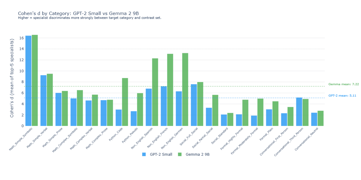 Feature population overlap
While H1 primarily examines specialist feature behaviors, I additionally included an examination of overlap in the top 20 most active feature population (regardless of whether those features fit my specialist definition) for each model.
Key takeaway: Gemma displays a far denser activation pattern, compared to GPT-2 Small. Gemma activates a substantially larger fraction of its feature vocabulary in response to any given text sample (~7-38% vs. ~1% for GPT-2), resulting in a correspondingly larger pool of shared active features across different surface forms and resulting in materially higher feature population overlap at both the top-5 and top-20 thresholds. These results are shown in Figure 4.
Figure 4: Feature population overlap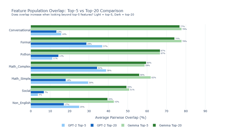
Sparsity rankings
Finally, for each model, I calculated L0 sparsity (the number of features activated by a given text sample) for all topic + form combinations. As shown in Figure 5 below, when I sorted those topic + form combinations by the number of features activated, that categorical ranking was highly consistent across both models (ρ = 0.87).
Key takeaway: The relative density (the number of features activated by each topic + form combination, compared to the other combinations) was consistent across both models, despite Gemma having far more active features overall. This indicates that syntax, not semantics, determines activation shape at both scales, further supporting the syntax-centric H1 conclusion.
Figure 5: Sparsity rankings by topic + form
H2: Overall representational geometry clusters by topic (both models)
The second avenue of analysis focused not on specialist features, but rather, on the overall representational geometry utilized by GPT-2 Small and Gemma 2 9b. To thoroughly examine this topic, I used 4 complementary analyses (cosine similarity, Spearman ranking, PCA, and silhouette). All four metrics demonstrated clear semantic-based clustering in both models. While not central to the hypothesis, I also found that this topic-based clustering emerged in earlier layers of GPT-2, compared to Gemma.
Cosine similarity
The primary means of measuring whether each model’s overall representation was primarily syntactically- or semantically-based was via cosine analysis. By comparing the cosine similarity of text pairs with the same meaning but different surface features vs. text pairs with entirely different meanings, we are able to gain a sense of the broad organization of those items within the model’s broader high-dimensional vector space.
Key takeaway: Both GPT-2 Small and Gemma 2 9b demonstrate clear topic-based clustering. Figure 6 shows that for each model, cosine similarity for same-topic, different-form pairs exceeded different topic pairs (0.53 vs. 0.14 for GPT-2 Small and 0.93 vs. 0.80 for Gemma).
Gemma’s much higher overall feature activation levels and a denser representational structure explains that model’s reduced gap between the topic-based and cross-topic cosine similarities). Figure 7 and Figure 8 show the complete pairwise cosine similarity results for each model. Importantly, Gemma's smaller gap between topic- and form-based clustering does not indicate a relative weakness in topic-based clustering. Instead, it reflects overall compression of Gemma's representational structure due to its denser activation patterns. In fact, the PCA analysis in Figure 15 below suggests Gemma's topic-based organization is actually stronger than GPT-2 Small's.
Figure 6: Cosine analysis summary
Figure 7: Cosine similarities - GPT-2 Small
Figure 8: Cosine similarities - Gemma 2 9b
Spearman rank
Additionally, I calculated a Spearman rank correlation coefficient (ρ) to determine the degree to which pairwise similarities were maintained in GPT-2 Small vs. Gemma 2 9b. The initial results of this analysis, shown in Figure 9 failed to show a meaningful pattern due to Gemma 2 displaying much higher cosine similarity values across the board.
Figure 9: Pairwise cosine similarities, uncorrected for differences in overall cosine similarity levels
To control for Gemma’s much higher cosine similarity values across the board (visible when comparing the values in figures 10 and 11), I utilized a rank-transformed approach that compared, for each model, the rankings of each text pair’s similarity, relative to other text pairs. Thus, I was able to see, for each model, which pairs were more similar to one another. Plotting those rankings in Figure 10 thus allowed me to see, for each pair, the similarity in GPT-2 vs. Gemma, controlling for differences in the overall scale of the cosine metrics involved. This plot shows that both models, despite their ~70x difference in scale, utilize a similar representational structure, and generally “agree” which of the matched pairs are most similar to one another.
Key takeaway: Spearman ranking, once corrected for Gemma’s much denser representational structure, suggests both models utilize a similar, topic-based overall representational structure.
Figure 10: Pairwise cosine similarities, normalized for differences in overall cosine similarity levels
PCA Analysis
Figure 11 shows GPT-2 Small’s representational geometry, including the aforementioned topic-based clustering. As discussed in the Phase 2 analysis and shown in Figure 12, one can see that some topics (such as Social and Conversational) are tightly clustered, while others (such as Math and Python) are more loosely-clustered. These results make sense in light of the aforementioned H1 findings that symbolic notation generally results in more active specialist features, since these specialists pull those text samples far out along a unique axis in high-dimensional space, resulting in greater variance among the text samples, manifested in their larger PCA spread.
Figure 11: PCA Analysis - GPT-2 Small
Figure 12: PCA Variance - GPT-2 Small
The PCA results for Gemma 2 9b, shown in Figure 13 and Figure 14 below, also demonstrate topic-based clustering, albeit with key differences in both the shape of the spread and which categories showed the most variance in their spread. One potential explanation for Gemma’s broader, fan-shaped PCA spread could be its denser activation structure, compared to GPT-2 Small. Since far more of the total Gemma feature set activates on a given text, compared to GPT-2, the opportunities for unique vectors are many and varied. Furthermore, the change in which topic categories have the most PCA variance is linked to Gemma’s strengths relative to GPT-2 Small. Gemma’s relatively high variance in the “Non-English” categories are likely connected to the combined effects of the following:
Figure 13: PCA Analysis - Gemma 2 9b
Figure 14: PCA Variance - Gemma 2 9b
Key takeaway: PCA analysis demonstrates clear semantic-based clustering in both models. Despite both utilizing a topic-centric overall representational structure, there exist key differences between the models in terms of the shape of those topic clusters (Gemma fan-shaped clustering is potentially indicative of its greater degree of shared features) and their relative topic-level strengths (Gemma is stronger in Python, for example).
Silhouette analysis
To augment the understanding of each model’s clustering behavior, I additionally performed a Silhouette analysis, which measured each sample text’s similarity to other texts with either the same topic (yielding the topic-based silhouette score) or the same form (yielding the form-based silhouette scores), compared to other, unrelated combinations.
Key takeaway: The results shown in Figure 15 demonstrate that for both models, the topic-based silhouette scores were greater than their form-based silhouette scores, confirming the topic-based clustering observed in the aforementioned PCA analysis.
Figure 15: Silhouette scores
Figure 16: Detailed, per-text silhouette scores
Figure 17: Topic-based silhouette scores
Figure 18: Nearest neighbor analysis - GPT-2 Small
Figure 19: Nearest neighbor analysis - Gemma 2 9b
Timing of clustering emergence
Finally, while not directly related to the geometry of the models' representational structure, I examined when the aforementioned topic-based clustering emerged in each model. To enable comparison across models with different total depths, layer position is normalized to a 0-to-1 scale, where 0 represents the input and 1 represents the final layer. As shown in Figure 20, GPT-2 Small exhibited topic-based clustering in much earlier layers, compared to Gemma.
Figure 20: Timing of topic-based clustering, by model layer
H3: Specialist activation levels affect output and model confidence
The third primary line of analysis performed explored the relationship between feature activation levels and each model’s output and its confidence in that output. This was approached from the following two perspectives:
As with H2, I utilized multiple complementary analyses to examine this topic (binary completions (activation vs. completion accuracy), cloze (activation vs. model confidence), and feature ablation (causal linkage between activation and completion accuracy). All three analyses pointed in the same direction, suggesting a clear linkage between feature activation and model behavior, in terms of both output and confidence, that varied widely by topic and model layer.
Binary completions
One of the lingering questions from Phase 2 of this series was whether specialist activation levels were related to a model’s generative abilities. To test this, I first used an LLM to generate 264 math completions (88 problems x 3 surface forms) and 96 non-math completions (12 problems × 3 forms for formal English and Non-English, and 12 problems × 2 forms for Python). Then, using point-biserial correlation, I compared the activation level of the relevant topic + surface form specialist to the model’s ability to answer the completion correctly.
Critically, this analysis was done across all the layers tested in each model. This proved a critical nuance, because while there exists minimal correlation between specialist feature activation and model accuracy at the last layer of each model, that changes for some topics at other layers throughout the models as the results below illustrate.
Key takeaway: Specialist activation is linked to model accuracy, but only in relation to the math topic’s various surface forms, and only at intermediate model layers, as shown in Figure 21 and Figure 22.
Each model’s final layer showed minimal linkage between specialist activation levels and completion accuracy (only 2 of the 8 topic + model combinations reached statistical significance and even in those cases, specialist activation only explained < 3% of the model’s ability to perform the completions accurately.
Figure 21: Specialist activation vs. completion accuracy (significant results)
Figure 22: Significance of specialist activation vs. completion accuracy
Cloze analysis
To augment the understanding provided by the aforementioned binary completion that looked for correlation between specialist activation and competition accuracy, I also performed cloze analysis, which looked for correlation between specialist activation and the model’s confidence in its answer, regardless of that answer’s accuracy. Because model confidence is a continuous function, as opposed to the binary nature completion accuracy (i.e. the answer must either be correct or incorrect), my cloze testing provided a more nuanced view, compared to the binary testing.
More specifically, the three metrics measured by this cloze analysis were the following:
Key takeaway: Similar to the binary completion analysis, feature activation levels showed statistically significant correlation with model confidence, primarily with regards to math’s various surface forms at Gemma’s intermediate layers, as shown in Figure 23, Figure 24, and Figure 25. As with the binary accuracy tests, it should be noted that this is a measure of correlation and not necessarily causation, between specialist activation and model behavior.
Figure 23: Specialist activation vs. model confidence (significant results in ≥ 2/3 metrics)
Figure 25: Significance of specialist activation vs. model confidence (Gemma 2)
Feature ablation
While the aforementioned binary accuracy and cloze analyses looked for correlation between specialist activation and model behavior, those results do not prove causation. For this reason, I added feature ablation testing in which the activation levels of the relevant features for each topic + surface form combination were artificially zeroed-out (ablated) to measure the resulting change in model behavior in terms of both confidence in output and changes in actual output (i.e. “flip rate”).
Key takeaway: The ablation results in Figure 26 and Figure 27 show model steerability by each topic + form combination and model layer. Once again, the devil is in the details: while steerability based on final layer intervention is limited, more surgical interventions across the model’s layer opens the door to significantly greater model control, particularly in the math and non-English topics for both models.
This topic- and layer-specific approach shifts the question from “is model X more steerable than model Y?” to a far more interesting, if complex question of “under what conditions is model X more steerable than model Y?” My results suggest that in general, GPT-2 is more steerable than Gemma when dealing with math text, while Gemma is more steerable when dealing with non-English text.
Figure 26: Effect of ablation on model flip rate by topic + surface form and layer
Figure 27: Effect of ablation on model confidence by topic + surface form and layer
V. Implications for AI safety
Effective steering requires surgical, layer-specific interventions
One of the primary motivations for embarking on this line of analysis was to better understand and articulate the relationship between model input, feature activation, and model output. This is the quest of mechanistic interpretation: to understand and control the model’s internal representational mechanics in such a way that it enables new and more effective ways of controlling model output.
This analysis shows, in no uncertain terms, that this kind of model manipulation is easier said than done. For both models tested, my initial, aggregated analysis was discouraging; it suggested that my ablation efforts had very minimal effects, if any, on the model’s output.
It was only after disaggregating that consolidated output did it become clear that effective interventions need to be surgical in nature. The specialist features identified in my analysis allowed me to steer each model, but that steerability varied greatly by topic + form combination and by model layer. Flip rates for GPT-2 and Gemma, for example, peaked at ~58% (non-English + German, layer 10) and ~91% (non-English + Spanish, layer 37), respectively. Conversely flip rates for both models were at or near zero for all surface forms of formal English, regardless of model layer.
The implications for model steerability are clear: effective steering via manipulation of specialist activation requires a deep understanding of both (a) what specialists to manipulate for each topic + surface form, and (b) at what layer to execute that manipulation. Furthermore, the idea of one model being generally more or less steerable than another model is less helpful than an understanding of each model’s topic-level steerability using correctly timed interventions. As mentioned above, the results of this analysis find that at comparable model layers, GPT-2 seems generally more steerable than Gemma when it comes to math content, while Gemma is generally more steerable than GPT-2 when it comes to Python code.
Confidence is easier to change, relative to output
Comparing the disaggregated effects of ablation on model output and confidence (Figures 25 and 26, respectively), we can see that the effects of ablation on confidence were generally much greater than the corresponding effects on model output. The reason for this is likely definitional. Since confidence reflects the relative probability of the model’s top-ranked token, relative to all other alternative tokens, a small nudge to the probabilities assigned to those alternative tokens can have a large effect on model confidence. Changing the model’s output, on the other hand, is a much higher bar. It requires a change to probabilities great enough that an alternate token completely overtakes the prior token associated with the highest relative probability.
Since steerability is ultimately about affecting model output in ways that make model outputs more reliable and socially beneficial, the confidence/output gap revealed here is a cautionary finding: the relative ease of shifting model confidence without changing actual output means that interventions which appear to be working by affecting measurable changes in model confidence confidence may be doing little or nothing to change what the model actually says. A safety intervention that looks effective when measured by confidence shifts may fail entirely when measured by the stricter standard of whether the model's output actually changed.
VI. Appendix
Figure A: Phase 3 matched pairs
Topic
Form
Sample Texts
Math (Simple)
Symbolic
• 8-3
• 5x3
• 3^2
Math (Simple)
Verbal
• Eight minus three
• Five times three
• Three squared
Math (Simple)
Prose
• Three less than eight
• Five multiplied by three
• Three to the power of two
Math (Complex)
Symbolic
• sin²(θ) + cos²(θ) = 1
• ∫x² dx = x³/3 + C
• d/dx(x²) = 2x
Math (Complex)
Verbal
• Sine squared theta plus cosine squared theta equals one
• The integral of x squared dx equals x cubed over three plus C
• The derivative of x squared equals two x
Math (Complex)
Prose
• The square of the sine of theta plus the square of the cosine of theta equals one
• The integral of x squared with respect to x is x cubed divided by three plus a constant
• The derivative with respect to x of x squared is two times x
Python
Code
• def add(x, y): return x + y
• for i in range(10):
• if x > 0: return True
Python
Pseudocode
• Define function add that takes x and y and returns x plus y
• Loop through numbers zero to nine
• If x is greater than zero then return true
Non-English
Spanish
• Hola, ¿cómo estás?
• Buenos días
• Gracias
Non-English
French
• Bonjour, comment ça va?
• Bonjour
• Merci
Non-English
German
• Hallo, wie geht es dir?
• Guten Morgen
• Danke
Social
Full Social
• omg that's so funny 😂😂😂
• this slaps fr fr 🔥🎵
• just got coffee ☕ feeling good ✨
Social
Partial Social
• omg thats so funny
• this slaps fr fr
• just got coffee feeling good
Social
Standard
• That's very funny
• This is really good
• I just got coffee and I feel good
Formal
Highly Formal
• The phenomenon was observed under controlled laboratory conditions.
• Pursuant to Article 12, Section 3 of the aforementioned statute.
• The results indicate a statistically significant correlation (p < 0.05).
Formal
Moderately Formal
• We observed the phenomenon in controlled lab conditions.
• According to Article 12, Section 3 of the law.
• The results show a significant correlation.
Formal
Plain
• We saw this happen in the lab
• Based on what the law says.
• The results show a real connection.
Conversational
First Person
• I think the meeting went pretty well today.
• I'm planning a trip to Japan.
• I need to finish this project by Friday.
Conversational
Third Person
• She thinks the meeting went pretty well today.
• He's planning a trip to Japan.
• They need to finish this project by Friday.
Conversational
Neutral
• The meeting seems to have gone well today.
• There are plans for a trip to Japan.
• The project needs to be finished by Friday.
Figure B: Phase 3 Math Completion Tasks (Selected Examples)
Category
Form
Prompt
Expected
Addition
Symbolic
2 + 2 =
4
Addition
Verbal
two plus two equals
4
Multiplication
Symbolic
6 * 7 =
42
Multiplication
Verbal
six times seven equals
42
Trigonometry
Symbolic
sin²(θ) + cos²(θ) =
1
Trigonometry
Verbal
sine squared theta plus cosine squared theta equals
1
Calculus
Symbolic
d/dx(x²) =
2x
Algebra
Symbolic
3x + 7 = 22, x =
5
Algebra
Verbal
if three x plus seven equals twenty-two, then x equals
5
Logarithms
Symbolic
log₂(64) =
6
Logarithms
Verbal
the base two logarithm of sixty-four equals
6
Negative-base exponents
Symbolic
(-2)^5 =
-32
Negative-base exponents
Verbal
What is negative two raised to the fifth power? The answer is
-32
Modular arithmetic
Symbolic
17 mod 5 =
2
Modular arithmetic
Verbal
What is the remainder when seventeen is divided by five? The answer is
2
Fraction arithmetic
Symbolic
3/4 + 1/2 =
5/4
Fraction arithmetic
Verbal
What is three-quarters plus one-half? The answer is
5/4
Nested operations
Symbolic
((2 + 3) × 4) - 7 =
13
Nested operations
Verbal
Add two and three, multiply by four, then subtract seven. The answer is
13
Figure C: H3 Non-Math Completion Tasks (Selected Examples)
Domain
Form
Sample Prompt
Expected
Python
Code
x = 5\ny = 10\nresult = x + y\nprint(result) # prints
15
Python
Pseudocode
# Set x to 5 and y to 10, then compute their sum\nx = 5\ny = 10\nresult = x + y\n# result equals
15
Python
Prose
In Python, if x = 5 and y = 10, then x + y evaluates to
15
Python
Code
def square(x):\n return x *
x
Python
Pseudocode
# Define a function that returns x squared\ndef square(x):\n return x *
x
Python
Prose
In Python, the keyword used to define a function is
def
Non-English
French
Bonjour, comment allez-
vous
Non-English
French
La tour Eiffel est à
Paris
Non-English
French
Deux plus trois font
cinq
Non-English
Spanish
Hola, ¿cómo estás? Muy
bien
Non-English
Spanish
Madrid es la capital de
España
Non-English
Spanish
Dos más tres son
cinco
Non-English
German
Guten Tag, wie geht es
Ihnen
Non-English
German
Berlin ist die Hauptstadt von
Deutschland
Non-English
German
Zwei plus drei ist
fünf
Formal
Highly formal
Historical records indicate that George Washington was born in the year
1732
Formal
Highly formal
The orbital period of the Earth around the Sun is approximately
365
Formal
Moderately formal
George Washington was born in
1732
Formal
Moderately formal
The Earth takes approximately
365
Formal
Casual
So Washington was born way back in
1732
Formal
Casual
It takes Earth approx. how long to go around the sun
365
Key metrics used
Specialist score
To help conceptualize and quantify the selectivity of a given SAE feature vis-a-vis the current category of sample texts, I used the following calculation,:
wherein:
It should be noted that the threshold activation level of 5.0 was chosen somewhat arbitrarily, but I do not suspect this is a significant issue, as it is applied uniformly across features and categories.
Critically, when calculating specialist features, the comparison set for each topic + form type includes all topic + form combinations except other forms of the same topic. For example, if the topic + form being analyzed is math_complex + symbolic, the contrasting sets would include python + code, python + pseudocode, non-English + French, non-English + German, etc. but not math_complex + verbal or math_complex + prose. This design was selected to avoid skewing the results, since a math_complex + symbolic feature may be more activated by other math_complex texts, relative to texts associated with an unrelated subject, such as Python or non-English text.
Gini coefficient:
One of the means I used to better understand the geometry of the top n most active features was via the calculation of a Gini coefficient for those features. The calculation was accomplished by sorting the activation levels and then comparing a weighted sum of activations (wherein each activation is weighted by its ranking) against its unweighted component. A Gini ranges from 0 to 1, wherein 0 indicates a perfectly equal distribution and 1 a perfectly unequal distribution (e.g. all activation resides in a single feature).
Concentration ratio:
To further enable an easy understanding of the top n feature geometry for a given text sample, I also calculated a simple concentration ratio that measured the total activation of the top n features for a given sample, relative to the total overall activation for that feature. While the concentration ratio thus calculated is similar to the Gini calculation described above, it tells a slightly different story. While the Gini helps one understand the geometry (i.e. the dispersion) of the top n features, relative to one another, the concentration ratio describes the prominence of those top n features relative to the overall activation associated with that sample text.
Feature Overlap (raw count)
Core to the matched pairs approach used in this analysis is the comparison of features activated among the various matched text pairs used. Feature overlap is a simple metric that counts the number of shared specialist features among the top 5 specialist features activated by two topic + surface form text samples.
For example, if math_simple + symbolic activates the following features: {1, 2, 3, 4, 5} and math_simple + verbal activates the following features: {2, 6, 7, 8, 9}, then the feature overlap would be 1, corresponding with feature #2.
Jaccard Similarity / Mean Jaccard:
Another metric used to measure the degree to feature overlap is Jaccard Similarity, which is essentially a scaled version of the feature overlap described above. It is calculated as follows:
wherein:
“A” and “B” represent the list of specialist features activated by two different surface form variations of the same concept. This value ranges from 0 (no specialist features shared between text sets A and B) and 1 (the same specialist features are activated by text sets A and B).
Using the same example shown for feature overlap, if math_simple + symbolic activates the following features: {1, 2, 3, 4, 5} and math_simple + verbal activates the following features: {2, 6, 7, 8, 9}, then the Jaccard Similarity would be 1/9 = 0.1
Cosine Similarity:
To quantify and compare each sample text’s representational geometry (e.g. the overlapping features and those features activations), I used cosine similarity for those pairs, which is calculated as follows:
wherein:
The cosine similarity ranges from 0 (no features in common between vectors A and B) to 1 (vectors for A and B have identical features and each feature has the same value).
This logic essentially extends the Jaccard Similarity described above. Whereas Jaccard Similarity looks at overlapping features in a binary sense (e.g. overlapping features with 0.1 activation are treated the same as overlapping features with 50 activation), cosine similarity accounts for that activation level, thus providing a richer picture of the representational space.
Cohen's d (Effect Size):
To create a simple, standardized measure of the difference in mean activation between the text samples in a given topic + form type and all contrasting topic + form types, I used Cohen’s d, which is calculated as follows:
wherein:
The reason for using this measurement is simple: to provide a scaled, comparable way to determine how “selective” a given feature’s activation is to a given topic + surface form combination vs. the activation of that same feature vis-a-vis the contrasting topic + surface form combinations.
Feature Population Overlap:
While the Jaccard Similarity described above measures overlap among the most selective features (i.e. those that activate most exclusively on a single category), Feature Population Overlap measures overlap among the most active features (i.e. those with the highest mean activation on a given category, regardless of whether they also activate on other categories).
For a given topic with multiple surface forms, I identified the top-N features by mean activation for each form, then calculated the percentage of those top-N features that appeared in the top-N lists of the other forms of the same topic.
This metric captures a fundamentally different question than Jaccard. Jaccard asks: "do the same features specialize on different forms of the same concept?" Feature Population Overlap asks: "do the same features activate strongly on different forms of the same concept?" A topic can have low Jaccard (different specialists per form) and high population overlap (many broadly-active features shared across forms) simultaneously. This outcome is exactly what is reflected in the results.
Silhouette Score:
To provide a more conservative, per-text measure of clustering quality beyond the cosine similarity analysis, I calculated silhouette scores for each individual text in the dataset. For a given text, the silhouette score measures how much closer that text's activation vector is to other texts in the same category versus texts in the nearest different category. It is calculated as:
wherein:
The silhouette score ranges from -1 to +1, where +1 means the text is much closer to its own category, 0 means it sits on the boundary between categories, and -1 means it is closer to a different category. I calculated silhouette scores using both topic labels and form labels, then compared the two: if topic silhouette exceeds form silhouette, texts cluster primarily by semantics, not syntax.
Point-Biserial Correlation (r):
To test whether specialist activation predicts task accuracy in the H3 behavioral tests, I used point-biserial correlation, which measures the relationship between a continuous variable (specialist activation level) and a binary variable (correct or incorrect). This is calculated as:
wherein:
A significant positive r would indicate that higher specialist activation is associated with the model producing a correct answer. A non-significant r would indicate that the specialist's activation, while it may reliably detect a surface form, does not predict whether the model succeeds at the task.
First-Token Log-Probability and Rank (Cloze Analysis):
Binary scoring (correct vs. incorrect) discards useful information in that it ignores how close to the correct answer the model was. For example, a model that assigns 40% probability to the correct answer and one that assigns 0.01% to the correct answer both score as "incorrect" in a simple binary correct / incorrect test. To recover this lost signal, I ran a single forward pass for each prompt and recorded two continuous measures of the model's confidence in whatever token it chose to generate first:
I then computed Spearman rank correlations between specialist activation and these confidence measures, so as to control for differences in overall activation levels between the models.
|Δ Log-Probability| (Ablation Effect Size):
To test whether specialist features have a causal influence on model output (as opposed to merely correlating with it), I performed ablation experiments. For each specialist feature, I zeroed out that feature's activation in the model's residual stream at hook_resid_pre, then re-ran the forward pass and recorded the model's new output distribution. The primary effect size metric is:
wherein log-prob_original and log-prob_ablated are the log-probabilities the model assigns to its originally-predicted first token before and after the ablation, respectively. A larger |Δ log-prob| indicates that the ablated feature had a greater causal influence on the model's confidence in its prediction.
I performed this ablation across all 4 SAE layers for each model, creating a matrix of specialist × layer conditions. Random features (selected without regard to domain) and cross-domain features (e.g. Python specialists tested on math prompts) served as controls to establish baseline noise levels.
Token Flip Rate:
A complementary and stricter measure of ablation impact, the token flip rate measures the percentage of prompts for which ablating a feature changed the model's top predicted token to a different token entirely. While |Δ log-prob| captures shifts in confidence, a model might become slightly less confident without actually changing its prediction. The token flip rate captures cases where the ablation changed what the model says, not just how confidently it says it.
KL Divergence:
To capture the full distributional impact of ablation beyond just the top predicted token, I also measured the Kullback-Leibler divergence between the model's original output distribution and its post-ablation output distribution across the entire vocabulary:
wherein P is the original output distribution and Q is the post-ablation distribution. A KL divergence of 0 means the distributions are identical (the ablation had no effect); larger values indicate greater distributional shift. This captures effects that neither |Δ log-prob| nor token flip rate would detect, such as redistribution of probability mass among non-top tokens.