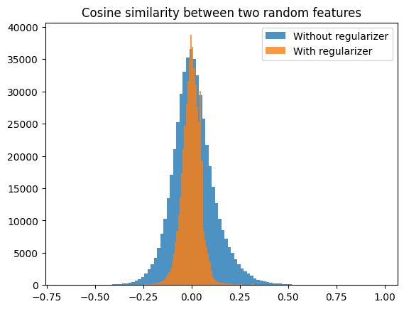
A quick and dirty first experiment with adding an orthogonality regularizer indicates that this can work without too much penalty on the reconstruction loss. I trained an SAE on the MLP output of a 1-layer model with dictionary size 8192 (16 times the MLP output size).
I trained this without the regularizer and got a reconstruction score of 0.846 at an L0 of ~17.
With the regularizer, I got a reconstruction score of 0.828 at an L0 of ~18.
Looking at the cosine similarities between neurons:
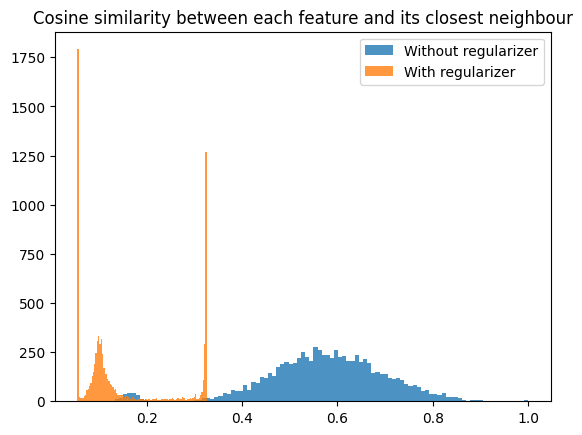
Interesting peaks around a cosine similarity of 0.3 and 0.05 there! Maybe (very speculative) that tells us something about the way the model encodes features in superposition?
The peaks at 0.05 and 0.3 are strange. What regulariser did you use? Also, could you check whether all features whose nearest neighbour has cosine similarity 0.3 have the same nearest neighbour (and likewise for 0.05)?
I expect the 0.05 peak might be the minimum cosine similarity if you want to distribute 8192 vectors over a 512-dimensional space uniformly? I used a bit of a weird regularizer where I penalized:
mean cosine similarity + mean max cosine similarity + max max cosine similarity
I will check later whether the 0.3 peak all have the same neighbour.
Nice, that's promising! It would also be interesting to see how those peaks are affected when you retrain the SAE both on the same target model and on different target models.
In the limit of infinite SAE width and infinite (iid) training data, you can get perfect reconstruction and perfect sparsity (both L0 and L1). We can think of this as maximal feature splitting. Obviously, this is undesirable, because you've discarded all of the structure present in your data.
Therefore, reconstruction and sparsity aren't exactly the thing we most fundamentally care about. It just happens to do something reasonable at practical scales. However, that doesn't mean we have to throw it out - we might hope that it gives us enough of a foothold in practice.
In particular, the maximal feature splitting case requires exponentially many latents. We might believe that in practice, on the spectrum from splitting too little (polysemanticity) to splitting too much, erring on the side of splitting too much is preferable, because we can still do circuit finding and so on if we artificially cut some existing features into smaller pieces.
Regarding achieving perfect reconstruction and perfect sparsity in the limit, I was also thinking along those lines i.e. in the limit you could have a single neuron in the sparse layer for every possible input direction. However please correct me if I’m wrong but assuming the SAE has only one hidden layer then I don't think you could prevent neurons from activating for nearby input directions (unless all input directions had equal magnitude), so you'd end up with many neurons activating for any given input and thus imperfect sparsity.
Otherwise mostly agreed. Though as discussed, as well as making it necessary to figure out how to break apart feature combinations (as you said), feature splitting would also seem to incur the risk of less common “true features” not being represented even within combinations so those would get missed entirely.
This is a very good explanation of why SAE's incentivize feature combinatorics. Nice! I hadn't thought about the tradeoff between the MSE-reduction for learning a rare feature & the L1-reduction for learning a common feature combination.
Freezing already learned features to iteratively learn more and more features could work. In concrete details, I think you would:
1. Learn an initial SAE w/ a much lower L0 (higher l1-alpha) than normally desired.
2. Learn a new SAE to predict the residual of (1), so the MSE would be only on what (1) messed up predicting. The l1 would also only be on this new SAE (since the other is frozen). You would still learn a new decoder-bias which should just be added on to the old one.
3. Combine & repeat until desired losses are obtained
There are at least 3 hyperparameters here to tune:
L1-alpha (and do you keep it the same or try to have smaller number of features per iteration?), how many tokens to train on each (& I guess if you should repeat data?), & how many new features to add each iteration.
I believe the above should avoid problems. For example, suppose your first iteration perfectly reconstructs a datapoint, then the new SAE is incentivized to have low L1 but not activating at all for those datapoints.
Thanks! Yeah I think those steps make sense for the iterative process, but I'm not sure if you're proposing that would tackle the problem of feature combinations by itself? I'm still imagining it would require orthogonality regularisation with some weighting
I've been looking into your proposed solution (inspired by @Charlie Steiner 's comment). For small models (Pythia-70M is d_model=512) w/ 2k features doesn't take long to calculate naively, so it's viable for initial testing & algorithmic improvements can be stacked later.
There are a few choices regardless of optimal solution:
- Cos-sim of closest neighbor only or average of all vectors?
- If closest neighbor, should this be calculated as unique closest neighbor? (I've done hungarian algorithm before to calculate this). If not, we're penalizing features that are close (or more "central") to many other features more than others.
- Per batch, only a subset of features activate. Should the cos-sim only be on the features that activate? The orthogonality regularizer would be trading off L1 & MSE, so it might be too strong if it's calculated on all features.
- Gradient question: is there still gradient updates on the decoder weights of feature vectors that didn't activate.
- Loss function. Do we penalize high cos-sim more? There's also a base-random cos-sim of ~.2 for the 500x2k vectors.
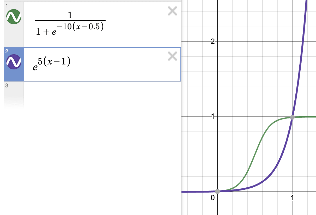
I'm currently thinking cos-sim of closest neighbor only, not unique & only on features that activate (we can also do ablations to check). For loss function, we could modify a sigmoid function:
This makes the loss centered between 0 & 1 & higher cos-sim penalized more & lower cos-sim penalized less.
Metrics:
During training, we can periodically check the max mean cos-sim (MMCS). This is the average cos-sim of the non-unique nearest neighbors. Alternatively pushing the histogram (histograms are nice, but harder to compare across runs in wandb). I would like to see normal (w/o an orthogonality regularizer) training run's histogram for setting the hyperparams for the loss function.
Algorithmic Improvements:
The wiki for Closest Pair of Points (h/t Oam) & Nearest neighbor search seem relevant if one computes the nearest neighbor to create an index as Charlie suggested.
Faiss seems SOTA AFAIK for fast nearest neighbors on a gpu although:
adding or searching a large number of vectors should be done in batches. This is not done automatically yet. Typical batch sizes are powers of two around 8192, see this example.
I believe this is for GPU-memory constraints.
I had trouble installing it using
conda install pytorch::faiss-gpu
but it works if you do
conda install -c pytorch -c nvidia faiss-gpu=1.7.4 mkl=2021 blas=1.0=mkl
I also was unsuccessful installing it w/ just pip w/o conda & conda is their offical supported way to install from here.
An additional note is that the cosine similarity is the dot-product for our case, since all feature vectors are normalized by default.
I'm currently ignoring the algorithmic improvements due to the additional complexity, but should be doable if it produces good results.
Testing it with Pythia-70M and few enough features to permit the naive calculation sounds like a great approach to start with.
Closest neighbour rather than average over all sounds sensible. I'm not certain what you mean by unique vs non-unique. If you're referring to situations where there may be several equally close closest neighbours then I think we can just take the mean cos-sim of those neighbours, so they all impact on the loss but the magnitude of the loss stays within the normal range.
Only on features that activate also sounds sensible, but the decoder weights of neurons that didn't activate would need to be allowed to update if they were the closest neighbours for neurons that did activate. Otherwise we could get situations where e.g. one neuron (neuron A) has encoder and decoder weights both pointing in sensible directions to capture a feature, but another neuron has decoder weights aligned with neuron A but has encoder weights occupying a remote region of activation space and thus rarely activates, causing its decoder weights to remain in that direction blocking neuron A if we don't allow it to update.
Yes I think we want to penalise high cos-sim more. The modified sigmoid flattens out as x->1 but the I think the purple function below does what we want.
Training with a negative orthogonality regulariser could be an option. I think vanilla SAEs already have plenty of geometrically aligned features (e.g. see @jacobcd52 's comment below). Depending on the purpose, another option to intentionally generate feature combinatorics could be to simply add together some of the features learnt by a vanilla SAE. If the individual features weren't combinations then their sums certainly would be.
I'll be very interested to see results and am happy to help with interpreting them etc. Also more than happy to have a look at any code.
Additionally, we can train w/ a negative orthogonality regularizer for the purpose of intentionally generating feature-combinatorics. In other words, we train for the features to point in more of the same direction to at least generate for-sure examples of feature combination.
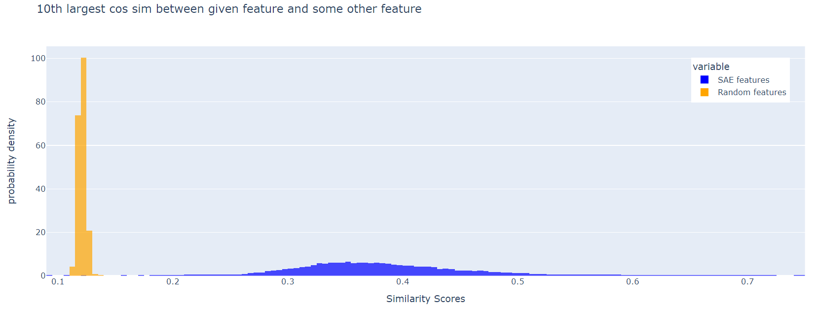
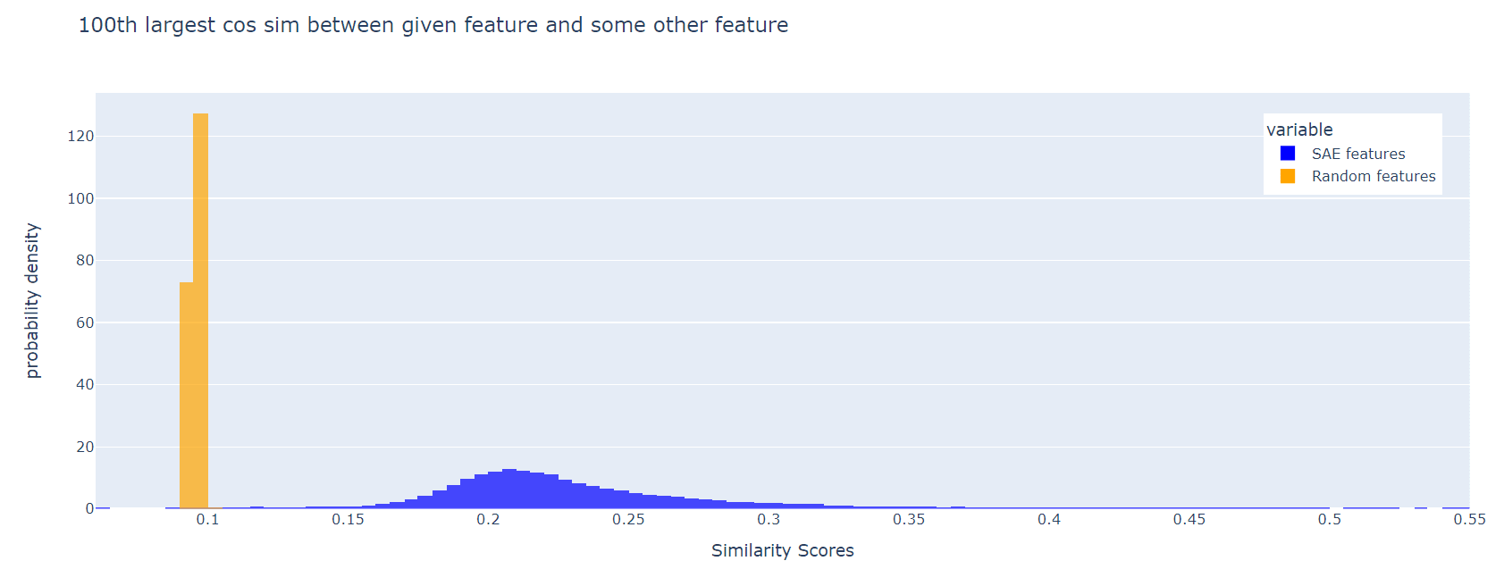
For each SAE feature (i.e. each column of W_dec), we can look for a distinct feature with the maximum cosine similarity to the first. Here is a histogram of these max cos sims, for Joseph Bloom's SAE trained at resid_pre, layer 10 in gpt2-small. The corresponding plot for random features is shown for comparison:
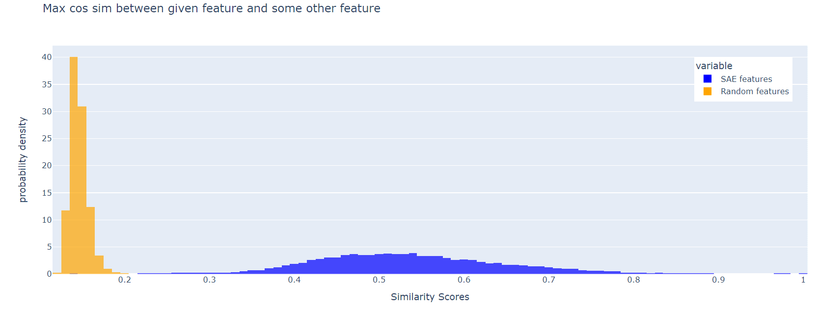
The SAE features are much less orthogonal than the random ones. This effect persists if, instead of the maximum cosine similarity, we look at the 10th largest, or the 100th largest:
I think it's a good idea to include a loss term to incentivise feature orthogonality.
I agree with pretty much all these points. This problem has motivated some work I have been doing and has been pretty relevant to think well about and test so I made some toy models of the situation.
This is a minimal proof of concept example I had lying around, and insufficient to prove this will happen in larger model, but definitely shows that composite features are a possible outcome and validates what you're saying:
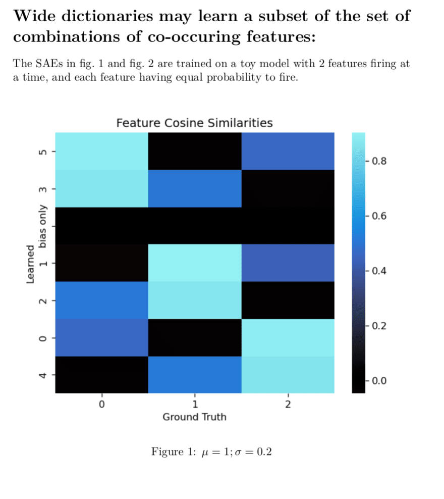
Here, it has not learned a single atomic feature.
All the true features are orthogonal which makes it easier to read the cosine-similarity heatmap.
and are mean and standard deviation of all features.
Note on "bias only" on the y-axis: The "bias only" entry in the learned features is the cosine similarity of the decoder bias with the ground truth features. It's all zeros, because I disabled the bias for this run to make the decoder weights more directly interpretable. otherwise, in such a small model it'll use the bias to do tricky things which also make the graph much less readable. We know the features are centered around the origin in this toy so zeroing the bias seems fine to do.
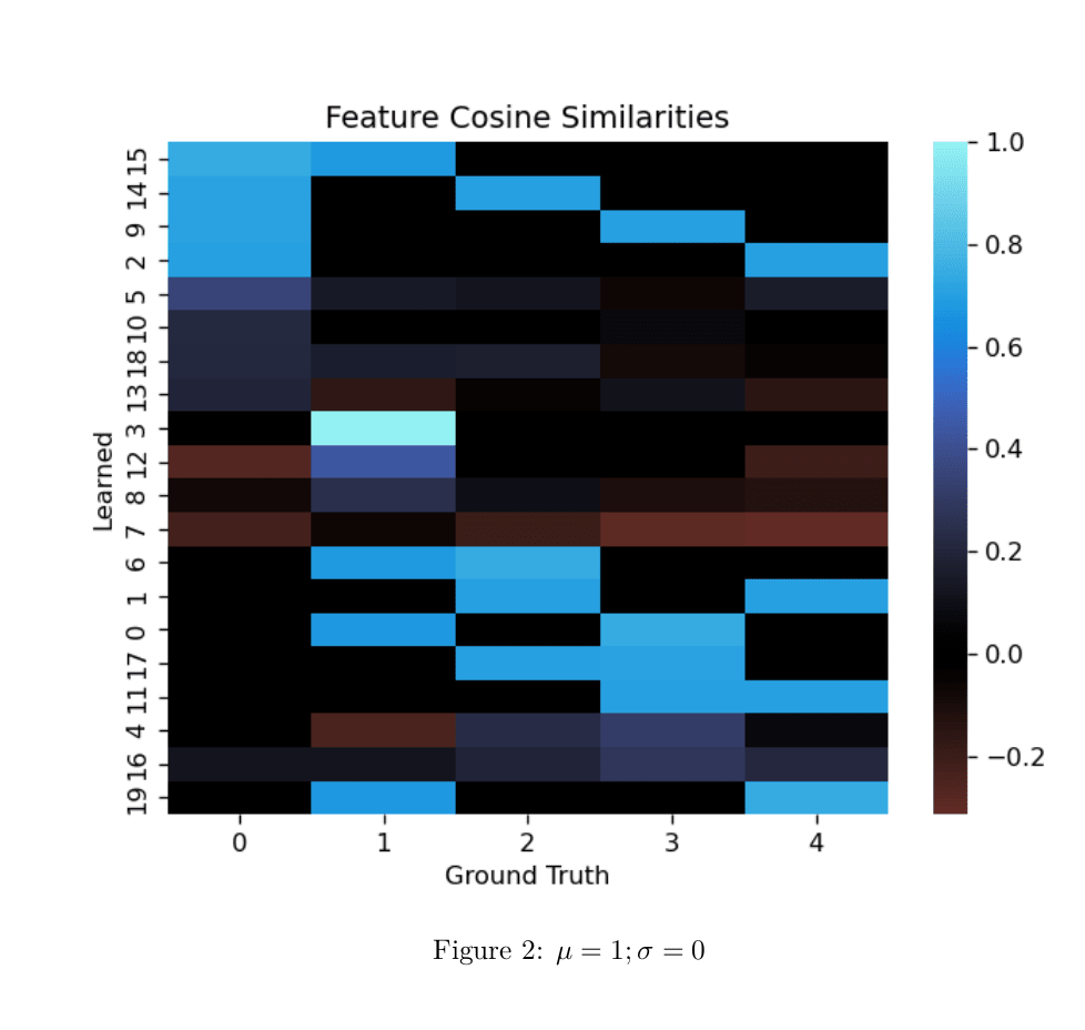
Edit: Remembered I have a larger example of the phenomena. Same setup as above.
This looks interesting. I'm having a difficult time understanding the results though. It would be great to see a more detailed write up!
Quadratic complexity isn't that bad, if this is useful. If your feature vectors are normalized you can do it faster by taking a matrix product of the weights "the big way" and just penalizing the trace for being far from ones or zeros. I think?
Feature vector normalization is itself an examble of a quadratic thing that makes it in.
Even for a fairly small target model we might want to discover e.g. 100K features and and the input vectors might be e.g. 768D. That's a lot of work to compute that matrix!
Hm. Okay, I remembered a better way to improve efficiency: neighbor lists. For each feature, remember a list of who its closest neighbors are, and just compute your "closeness loss" by calculating dot products in that list.
The neighbor list itself can either be recomputed once in a while using the naive method, or you can accelerate the neighbor list recomputation by keeping more coarse-grained track of where features are in activation-space.
Thanks, I mentioned this as a potential way forward for tackling quadratic complexity in my edit at the end of the post.
A potential approach to tackle this could be to aim to discover features in smaller batches. After each batch of discovered features finishes learning we could freeze them and only calculate the orthogonality regularisation within the next batch, as well as between the next batch and the frozen features. Importantly we wouldn’t need to apply the regularisation within the already discovered features.
Wouldn't this still be quadratic?
If n is the number of feature we're trying to discover and m is the number of features in each batch, then I'm thinking the naive approach is O(n^2) while the batch approach would be O(m^2 + mn). Still quadratic in m, but we would have m<<n
The SAE could learn to represent the true features, A & B, as the left graph, so the orthogonal regularizer would help. When you say the SAE would learn inhibitory weights*, I'm imagining the graph on the right; however, these features are mostly orthogonal to eachother meaning the proposed solution won't work AFAIK.
(Also, would be the regularizer be abs(cos_sim(x,x'))?)
*In this example this is because the encoder would need inhibitory weights to e.g. prevent neuron 1 from activating when both neurons 1 & 2 are present as we will discuss shortly.
yeah I was thinking abs(cos_sim(x,x'))
I'm not sure what you're getting at regarding the inhibitory weights as the image link is broken
Thanks for saying the link is broken!
If the True Features are located at:
A: (0,1)
B: (1,0)
[So A^B: (1,1)]
Given 3 SAE hidden-dimensions, a ReLU & bias, the model could learn 3 sparse features
1. A^~B (-1, 1)
2. A^B (1,1)
3. ~A^B(1,-1)
that output 1-hot vectors for each feature. These are also are orthogonal to each other.
Concretely:
import torch
W = torch.tensor([[-1, 1],[1,1],[1,-1]])
x = torch.tensor([[0,1], [1,1],[1,0]])
b = torch.tensor([0, -1, 0])
y = torch.nn.functional.relu(x@W.T + b)
It might be worth pointing out ‘ICA with Reconstruction Cost for Efficient Overcomplete Feature Learning’ (@NeurIPS 2011) which argues that the reconstruction cost |WW^Tx - x| can be used as a form of soft orthonormalization loss.
https://proceedings.neurips.cc/paper/2011/file/233509073ed3432027d48b1a83f5fbd2-Paper.pdf
I'm confused about your three-dimensional example and would appreciate more mathematical detail.
Call the feature directions f1, f2, f3.
Suppose SAE hidden neurons 1,2 and 3 read off the components along f1, f2, and f1+f2, respectively. You claim that in some cases this may achieve lower L1 loss than reading off the f1, f2, f3 components.
[note: the component of a vector X along f1+f2 here refers to 1/2 * (f1+f2) \cdot X]
Can you write down the encoder biases that would achieve this loss reduction? Note that e.g. when the input is f1, there is a component of 1/2 along f1+f2, so you need a bias < -1/2 on neuron 3 to avoid screwing up the reconstruction.
Hey Jacob! My comment has a coded example with biases:
import torch
W = torch.tensor([[-1, 1],[1,1],[1,-1]])
x = torch.tensor([[0,1], [1,1],[1,0]])
b = torch.tensor([0, -1, 0])
y = torch.nn.functional.relu(x@W.T + b)
This is for the encoder, where y will be the identity (which is sparse for the hidden dimension).
I was confused until I realized that the "sparsity" that this post is referring to is activation sparsity not the more common weight sparsity that you get from L1 penalization of weights.
Thanks to Joseph Bloom and James Oldfield for giving feedback on drafts which helped improve the post
In this post I'll discuss an apparent limitation of sparse autoencoders (SAEs) in their current formulation as they are applied to discovering the latent features within AI models such as transformer-based LLMs. In brief, I'll cover the following:
Rough definition of "true features"
We intend for SAEs to discover the "true features" (a term I'm borrowing from Anthropic's SAE paper) used by the target model e.g. a transformer-based LLM. There isn't a universally accepted definition of what "true features" are, but for now I'll use the term somewhat loosely to refer to something like:
There may be other ways of thinking about features but this should give us enough to work with for our current purposes.
Why SAEs are incentivised to discover combinations of features rather than individual features
Consider a toy setup where one of the hidden layers in the target model has 3 "true features" represented by the following directions in its activation space:
Additionally, suppose that feature 1 and feature 2 occur far more frequently than feature 3, and that all features can potentially co-occur in a given activation vector. For the sake of simplicity let's also suppose for now that when features 1 & 2 occur together they tend to both activate with some roughly fixed proportions. For example, an activation vector in which both features 1 and 2 are present (but not feature 3) might look like the following:
Now suppose we train an SAE with 3 neurons in the sparse layer on activation vectors from this hidden layer such as the one above. The desirable outcome is that each of the 3 neurons in the sparse layer learns one of the 3 "true features". If this happens then the directions learnt by SAE would mirror the directions of the "true features" in the target model, looking something like:
However depending on the respective frequencies of feature 3 vs features 1 & 2, as well as the value of the L1 regularisation weight, I will argue shortly that what may happen is that two of the neurons learn to detect when each of features 1 & 2 respectively occur by themselves, while the third neuron learns to detect when they both occur together. In this case the directions discovered by the SAE would look something like:
Note that for clarity I'm assuming that the SAE is trained with untied encoder/decoder weights and that it would be the decoder weights which would contain these directions and not the encoder. In this example this is because the encoder would need inhibitory weights to e.g. prevent neuron 1 from activating when both neurons 1 & 2 are present as we will discuss shortly. Also see Nanda's discussion and findings here on SAE encoder/decoder weight tying.
There are two problems with the directions hypothetically learnt by the SAE here. One problem is that feature 3 hasn't been represented at all, so we wouldn't know anything about that feature from this SAE. The second problem is that one of the neurons has learnt a combination of features which may confuse us in our attempts to understand what the "true features" are. If we tried to interpret what causes neuron 3 to activate we may still get what seems like a reasonable human-understandable interpretation and it isn't clear how we could tell which neurons correspond to individual "true features" and which correspond to combinations thereof. If there is a way then it would require additional effort/machinery.
Now let's discuss why the SAE might learn these directions instead of the ones corresponding to the 3 "true features". The key point is that by learning these directions it is able to achieve greater sparsity on average. If it learnt the directions we want it to learn then when features 1 & 2 occur together the SAE would need to activate both of the two neurons corresponding to these features:
However if neuron 3 learns the combination of features 1&2 then the SAE would only need to activate neuron 3, thus achieving greater sparsity:
Note that the encoder weights for these neurons would need to learn bias thresholds and in the case of neurons 1 & 2 inhibitory weights such that they only activate when the specific individual feature or combination thereof is active. There wouldn't be any sparsity gain if all 3 neurons activated when both features 1 & 2 are present.
The most obvious counterargument here is that failing to learn a neuron corresponding to feature 3 comes with the cost of increased reconstruction error when feature 3 is present. However if feature 3 is sufficiently rare compared with the combination of features 1 & 2 and the L1 regularisation weight is sufficiently high then the increased reconstruction error will be outweighed by the gain in sparsity. If we decrease the L1 regularisation weight then we may get feature 3 represented but we may also lose the sparse representations we're after, leaving us back at square one with polysemantic neurons. It isn't clear that there should exist a sweet spot for the L1 weight, and as we'll discuss shortly the ubiquity of feature splitting found in anthropic's SAE paper despite trying different L1 weights suggests there may not be an ideal sweet spot in practical settings. Any value for the L1 weight would likely be a compromise between learning monosemantic neurons and avoiding learning feature combinations.
Another counterargument is that we can simply increase the number of neurons in the sparse layer in order to capture rarer features as well as combinations of more common features. In this toy example, if we increase the width of the sparse layer to 4 neurons then feature 3 would presumably be represented. That is if we maintain the assumption that features 1 & 2 always co-activate with roughly the same proportions, allowing the single combination neuron to capture these co-occurences. In this case our learnt directions might look something like:
However if we relax this assumption, again depending on frequencies of feature activations, our SAE may end up using the extra capacity in the sparse layer to learn additional combination directions capturing differing proportions of activation levels of features 1 & 2. In this case the feature directions learnt by the SAE could look something like:
In this case the extra capacity is used to represent more common combinations at the expense of representing feature 3. With a realistic target model there would be many more "true features", many subsets of which would likely frequently co-occur with varying activation levels, which could result in a huge number of feature combination directions. Some of these combination directions will likely be sufficiently common compared with rarer individual features as to be prioritised by the SAE over said rarer individual features. But even if we increased the sparse layer width enough to capture all of these common feature combination directions along with all of the less common individual "true features", we would still face the problem of being swamped with feature combinations with often only subtly varying interpretations, making it more difficult to find the "true features".
Relation to feature splitting
We'll now look at some findings from Anthropic's SAE paper and discuss how they may be explained using the framework we've been developing. A surprising finding was that the "features" discovered by the SAEs they trained were often aligned with one another both conceptually and geometrically. I'm using "features" here to refer to interpretable directions found by the SAE which may or may not correspond to "true features" in the target model. For example two of the "features" they found had the following interpretations:
As well as being similar conceptually, they found that such "features" would also correspond to similar directions in activation space.
They found that this sort of phenomenon was ubiquitous in the "features" discovered by the SAEs they trained, with the "features" forming clusters of conceptual and geometric relatedness. Furthermore, they found that as they increased the width of the SAEs, the clusters would become more densely populated with increasingly nuanced distinctions between them.
They suggest that as they increase the width of the SAE, they may be converging on the "true features" which are represented in the target model. They hypothesise that these "true features" are even more densely packed and nuanced than the "features" they've found so far, and that the "features" they've found provide a sort of conceptual "summary" of the "true features". The narrower the SAE, the more coarse grained the summary. For example in the 512-width SAE they found a neuron which seemed to correspond to "'the' in mathematical prose", and in the 16,384 width SAE, they found one neuron which seemed to correspond to "'the' in the context of mathematics, especially complex analysis" and another neuron which seemed to correspond to "'the' in the context of mathematics, especially topology and abstract algebra". Notice how the neuron in the 512 width SAE provides a sort of summary for the 2 neurons in the 16,384 width SAE, and those may in turn provide summaries for the even more nuanced "true features".
However my theory is that this phenomenon is unlikely to be a reflection on the nature of the "true features". Rather, this phenomenon seems to be in line with what our earlier analysis would predict as a result of SAEs finding feature combinations and having more capacity to do so as the width is increased. Suppose the "true features" in a given layer of a target model include ones with interpretations along the lines of:
And suppose that the directions for these features are close to orthogonal. Note that they would be very unlikely to be completely orthogonal due to superposition, but we might expect the target model to attempt to make them as close to orthogonal as possible to minimise interference between features. So the "true feature" directions might look something like this:
Of course in reality the activation space would be far higher dimensional and there would be many more "true features".
Suppose that activation vectors from this layer frequently exhibit "the token 'the'" along with one (but not both) of the other "true features" being active. Then based on our earlier reasoning, we might expect some of the directions learnt by an SAE trained on activations from this layer to look something like:
Here we have 3 neurons that have learnt the individual feature directions + two more that have learnt commonly co-occurring combinations.
Note that they actually found hundreds of different "features" for "the in the context of []" for different contexts. Thus another possibility is that the "features" learnt by the SAE could look something like:
This would be possible if the SAE has learnt enough feature combinations so as to cover all of the combinations that the constituent individual "true features" are likely to appear in. This would preclude the need to learn the individual "true features" since all or most appearances of these features could be represented by one of the combination neurons.
Notice that since the feature combinations above share the feature "the token 'the'" as a component, they are aligned both conceptually and geometrically, as was the case with the 'features' discovered in the paper.
If we were to try to interpret neurons 1&2 without knowing the "true features" in the target model, just by looking at what activation vectors cause the neurons to activate, we might come up with interpretations similar to ones from the paper such as:
As for why the SAE features form clusters, one possibility is that this is a result of the existence of clusters of "true features" which tend to occur together in the same activation vectors. Perhaps there is a property of the data used to prompt the transformer target model whereby input sequences tend to pertain to a certain topic, and each topic has a set of features which are more likely to occur in that topic. The SAE is then more likely to learn feature combinations for these commonly co-occurring clusters of features.
Now let's explore why the "features" seem to "split", becoming increasingly specific. A narrow SAE could use its limited capacity to capture the most commonly occurring combinations along with the individual features. For example, if the "true features" include the following:
then we might expect a relatively narrow SAE to capture the combination, potentially along with capturing the individual features:
since this covers all mathematical prose, including topology and abstract algebra, and would thus likely occur more frequently than either of the sub-topics.
But a wider SAE might use its extra capacity to capture the less common combinations:
This could explain why features tend to get increasingly specific as the width increases and why features in narrower SAEs can be seen as summarising those found by wider SAEs.
Proposed solution
A naive idea for a solution to SAEs learning feature combinations could involve trying to adjust the width of the SAE to roughly match the number of "true features". One issue here is that we don't currently have any way to know how many "true features" we are trying to find. Even if we somehow knew the number of "true features", this approach would be unlikely to work due to the issue discussed earlier where some feature combinations may occur sufficiently frequently such that the sparsity gained by learning those combinations outweighs the reconstruction error incurred by not representing some of the rarer features.
Another idea could be to try tuning the sparse regularisation weight λ to avoid incentivising learning combinations of features. But reducing λ reduces the penalty for representing features by arbitrary directions in the SAE rather than individual neurons. As discussed earlier, it isn't clear that there ought to exist a sweet spot for λ to achieve sufficient sparsity while avoiding learning feature combinations instead of individual features. The ubiquity of the phenomenon of feature splitting observed in Anthropic's SAE paper despite trying a range of values for lambda suggest that such a sweet spot isn't likely to exist.
I propose including an additional regularisation term in the SAE loss to penalise geometric non-orthogonality of the feature directions discovered by the SAE. One way to formalise this loss could be as the sum of the absolute values of the cosine similarities between each pair of feature directions discovered in the activation space. Neel Nanda's findings here suggest that the decoder rather than the encoder weights are more likely to align with the feature direction as the encoder's goal is to detect the feature activations, which may involve compensating for interference with other features.
If we train SAEs on the same target model both with and without this additional regularisation term we can then investigate whether geometric orthogonality really is a reasonable prior for the "true feature" directions. If it isn't a reasonable prior then we would expect substantially worse reconstruction error. If it is a reasonable prior then we would expect it to discover features that weren't discovered by the vanilla SAE because it used up its capacity on learning feature combinations.
Another test could be to look for features which seem to correspond to the individual constituents of apparent composite features e.g. if the vanilla SAE discovered the feature "the token 'the' in the context of mathematical prose" then we can look for features in the SAE with orthogonality regularisation which seem to correspond to the constituent concepts "the current token is 'the'" and "the current context is mathematical prose". An interesting question would then be whether the direction for the feature "the token 'the' in the context of mathematical prose" is approximately a linear combination of the directions for the features "the current token is 'the'" and "the current context is mathematical prose". If we consistently find for different groups of features that the feature directions obey the expected arithmetic then it would seem reasonable to conclude that feature splitting is an artefact of SAEs rather than a reflection on the structure of the space of the "true features".
Depending on the weight of the orthogonality regularisation term we may still find that some feature combinations are discovered. Setting the weight too high may hinder the discovery of "true features" if they are sometimes somewhat aligned with one another while setting it too low would allow neurons to learn overlapping combinations of features, so this hyperparameter would require some tuning. It could also be beneficial to apply a non-linearity to the orthogonality loss to severely penalise more closely aligned feature directions whilst being more lenient on only slightly aligned feature directions, which could potentially be a more accurate reflection on the structure of the "true feature" directions.
Note that a naive implementation of this method would become extremely computationally intensive as we apply SAEs to larger target models with more "true features" and more dimensions in their activation vectors. The naive implementation to compute the orthogonality regularisation term would involve comparing every discovered feature direction to every other discovered feature direction. This would have quadratic computational complexity in the number of features we are trying to discover. A potential approach to tackle this could be to aim to discover features in smaller batches. After each batch of discovered features finishes learning we could freeze them and only calculate the orthogonality regularisation within the next batch, as well as between the next batch and the frozen features. Importantly we wouldn’t need to apply the regularisation within the already discovered features[1].
Citing this post
Chris_Leong correctly pointed out in the comments below that this batching algorithm would still have quadratic complexity overall. Something along the lines of neighbor lists as suggested by Charlie Steiner in the comments below could be a way forward. And perhaps having the already discovered 'frozen' features being stationary targets with the batching approach could be advantageous.