FFS has a different notion of causality, which is both weaker and stronger in important ways. FFS defines the history of an event to be the minimal set of factors which uniquely specify an element of . Then an event is thought of as "after" (written ) if the history of is a subset of the history of .
This makes one huge departure from Bayes nets: no information is allowed to be lost. If we have a system where directly causes , but there is some "noise" in which does not affect the downstream value of , then is not "before" .
Is this actually different from Bayes nets? Like let's say you have a probability distribution , but then you measure each variable with noise, , , . In that case the measurements won't satisfy , because will be dependent on even after conditioning on .
Yes there will be some special-cases where Bayes nets support it, e.g. if you've got only two variables , but these special cases rapidly fail as you have even slightly more complexity.
I was thinking about causality in terms of forced directional arrows in Bayes nets, rather than in terms of d-separation. I don't think your example as written is helpful because Bayes nets rely on the independence of variables to do causal inference: is equivalent to .
It's more important to think about cases like where causality can be inferred. If we change this to by adding noise then we still get a distribution satisfying (as and are still independent).
Even if we did have other nodes forcing (such as a node which is parent to , and another node which is parent to ), then I still don't think adding noise lets us swap the orders round.
On the other hand, there are certainly issues in Bayes nets of more elements, particularly the "diamond-shaped" net with arrows . Here adding noise does prevent effective temporal inference, since, if and are no longer d-separated by , we cannot prove from correlations alone that no information goes between them through .
I had forgotten about OEIS! Anyway Ithink the actual number might be 1577 rather than 1617 (this also gives no answers). I was only assuming agnosticism over factors in the overlap region if all pairs had factors, but I think that is missing some examples. My current guess is that any overlap region like should be agnostic iff all of the overlap regions "surrounding" it in the Venn diagram (, , , ) in this situation either have a factor present or agnostic. This gives the series 1, 2, 15, 1577, 3397521 (my computer has not spat out the next element). This also gives nothing on the OEIS.
My reasoning for this condition is that we should be able to "remove" an observable from the system without trouble. If we have an agnosticism, in the intersection , then we can only remove observable if this doesn't cause trouble for the new intersection , which is only true if we already have an factor in (or are agnostic about it).
Are you sure the "arrow forgetting" operation is correct?
You say there should be an arrow when
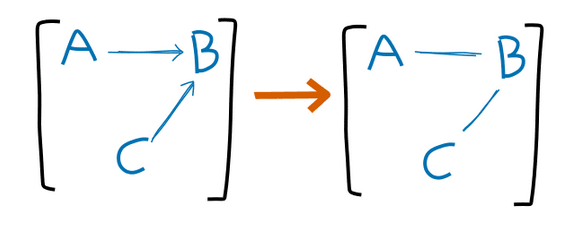
for all probability distributions over the elements of , the approximation of over is no worse than the approximation of over
wherein here, and . If we take a distribution in which , then is actually a worse approximation, because must hold in any distribution which can be expressed by a graph in right?
Also, I really appreciate the diagrams and visualizations throughout the post!
Thanks for the feedback. There's a condition which I assumed when writing this which I have realized is much stronger than I originally thought, and I think I should've devoted more time to thinking about its implications.
When I mentioned "no information being lost", what I meant is that in the interaction , each value (where is the domain of ) corresponds to only one value of . In terms of FFS, this means that each variable must be the maximally fine partition of the base set which is possible with that variable's set of factors.
Under these conditions, I am pretty sure that
I am confused about the last correspondence between Venn Diagram and BN equivalence class (this one: 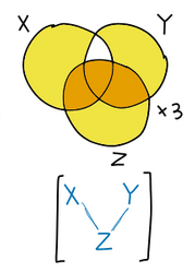
I was hoping I could produce a one-to-one mapping between diagrams of overlapping factors (from FFS) and Bayes nets. This is not possible, but instead I have been able to produce a similar mapping between factor overlap diagrams and sets of Bayes nets, subject to certain compatibility relationships.
Bayes Nets
The Bayes nets over some variables X can be thought of as a category of objects related by "bookkeeping" (and similar) relationships. To be more specific, we can say that a unique morphism exists between two Bayes nets Ni→Nj exists if and only if, for all probability distributions P over the elements of Ni, the approximation of Nj over P is no worse than the approximation of Ni over P. For two variables we need the Markov-chain-re-rooting and arrow-adding rules:
We could (with some effort) do three variables, but since there are three options for each pair of variables (A→B, A←B, no arrow) the number of Bayes nets over n variables is 312n(n−1). For n=3 this is 27. Let's draw in the adding-an-arrow and Markov-chain-re-rooting relationships:
As you can see it's a total goddamn mess! Even when we exclude the forbidden Bayes nets, ignore the identity morphisms (from an object to itself), use illicit double-headed arrows on the bottom layer, and also use "implied" arrows (i.e. don't bother with A→Cif we have A→B→C) we get a very confusing scenario!
To this problem, we will add another problem! But a problem which will lead us to a solution.
From Bayes Nets to Equivalence Classes
Say we have a mapping from a Finite Factored Set ontology to a Bayes net. This means we can apply a probability distribution over our factors to get a probability distribution over our downstream variables, with the condition that this must satisfy the Bayes net. The problem here is that many different Bayes nets will be satisfied by the probability distribution.
What we want is a one-to-one relationship (ideally). To improve this, we can start by grouping Bayes nets together under an equivalence relation. This is some relationship which has the following properties:
Reflexive: a∼a
Symmetric: a∼b⟺b∼a
Transitive: a∼b, b∼c⟹a∼c
We can define an equivalence relation over the category of Bayes nets over X trivially: Xi∼Xj⟺Xi→Xj∧Xj→Xi. For simpler Bayes nets, we can use undirected lines to make it easier to see what we are doing. As an example over our 3-element Bayes nets:
The square bracket notation [N] means an equivalence class and should be read as "The equivalence class containing N. On the right we've replaced our directed arrow with an undirected one. This is simply a change (perhaps abuse) of notation, which helps to remind us of the equivalence class that is present. We can do this for any Markov chain in our Bayes net, but we don't have to, especially when things get complicated.
Redrawing our map of the three-element Bayes nets:
Much nicer! Only 11 objects now! But we have made a critical mistake! We've assumed that we know all of the "bookkeeping" operations. We've missed one one. I think of this one as the "arrow forgetting" operation [1], and it makes more sense on equivalence classes:
I don't know the generalization of this to more than three elements. Our corrected category of equivalence classes looks like this:
Because of 2, we can define ≤ on our objects, such that NDis≥Ni≥NInd. Our choice of the direction of ≤ is such that the discrete Bayes net gives us the most information about the independence of variables. We say that Ni is finer than Nj if Ni≥Nj, because it encodes more information about the independence of variables.
Finite Factored Sets
FFS has a different notion of causality, which is both weaker and stronger in important ways. FFS defines the history of an event X to be the minimal set of factors which uniquely specify an element of X. Then an event Y is thought of as "after" X (written X≤Y) if the history of X is a subset of the history of Y.
This makes one huge departure from Bayes nets: no information is allowed to be lost. If we have a system where X directly causes Y, but there is some "noise" in X which does not affect the downstream value of Y, then X is not "before" Y. This is especially relevant when we are accessing measurements of X and Y, and not the world directly.
Now let us consider three variables, again X, Y and Z, and the factors making up their histories. We can use a Venn diagram to demonstrate the presence or absence of shared factors, and also write down the time ordering of X, Y, and Z according to FFS. I will call these "factor overlap diagrams".
Note that the networks in the middle column are not Bayes nets, they instead show which of our "downstream" variables depend on which factors.
I won't draw them out, but there are 27=128 different possible Venn diagrams we could draw here.
Mapping Them Together
This is where things become tricky. We might want to begin by noticing that we can ignore the three "outer" parts of the Venn diagram (in the drawings below I'll colour them a paler yellow) because Bayes nets are agnostic to additional factors as long as information is conserved.
This reduces us to just sixteen cases, and using symmetry this reduces to just eight.
Here we go! [2]
Ugh. Our relationship isn't one-to-one. It isn't even many-to-one. It's many-to-many. The problem is with the (lack of) specificity of equivalence classes. Just because a probability distribution satisfies one equivalence class, doesn't mean it can't also satisfy others. We can avoid this when one Bayes net is finer than the other, but because our ordering is only partial we cannot always define a total ordering.
From Equivalence Classes to Compatible Sets
We will define a set of Bayes nets over n variables as compatible if there exists some probability distribution which satisfies all of the Bayes nets, and no other Bayes nets over n variables. This generally means all of the Bayes nets in one or more equivalence classes, plus all of the Bayes nets in equivalence classes coarser than those. [3]
We designate all of the compatible sets of Bayes nets based on the equivalence classes they descend from. We can also define a partial ordering on the compatible sets by inclusion, i.e. N→M⟺N≥M⟺N⊇M. We note that our "finer" compatible sets contain more sets, therefore they impose more constraints on the underlying probability distribution.
We can also create some new notation to describe certain compatible sets:
This notation is unlikely to be ideal, but it does allow us to create the following diagram:
Now we have fifteen objects: four symmetric triples and three singletons. This is one less than our set of factor overlap diagrams. To make the connections one-to-one, we must merge two factor overlap diagrams. The choice is already made for us: two factor diagrams both map to the set containing just the indiscrete Bayes net. (An added benefit of moving to compatible sets is that it decreases any ominous resemblance present in diagram of equivalence classes)
We can make the following equivalence rule for our three elements: if h(Xi)∩h(Xj)≠{} ∀XjXj∈X then we are agnostic over whether ⋂{h(Xi)∀Xi∈X}={}. We'll continue to use pale yellow to denote agnosticism over the presence of elements in a Venn diagram.
We can draw the diagram of possible factor overlap diagrams. We can add arrows to denote whether a given factor overlap diagram contains factors in all of the locations of another one:
Hmm, looks familiar!
Thinking about compatible sets of Bayes nets allows us to think about the algebraic rules of Bayes nets more sensibly. If we notate the set of compatible sets of Bayes nets over n variables CSBn, we can think of rules like the Frankenstein rule as maps of the form CSBn×CSBn→CSBn i.e. taking two sets of Bayes nets (which are satisfied by a probability distribution) and then returning a new set of Bayes nets. In fact there will only be one general map of this form, which should contain all rules for combining Bayes nets over the same variables as a special case. The stitching rule can be thought of as a map of the form CSBl+m×CSBm+n→CSBl+m+n.
(Strictly speaking this might not be true, because we haven't made sure that our morphisms are mapped properly)
This might also relate to our ability to compute the factors of a distribution. It is computable which Bayes nets a distribution fits to, and therefore going from the relevant compatible set to a factor diagram should also be possible.
A few Illustrative Examples
What does it actually mean for certain distributions to obey multiple non-equivalent Bayes nets?
Example 3: X = temp in F, Y = temp in C, Z = phase of water. This satisfies two different Bayes equivalence classes, corresponding to a single compatible set.
Example 2: X = temp in F, Y = temp in C, Z = temp in K. All three depend on the same factor (actual physical temperature). This satisfies the following three equivalence classes:
Conjectures and Limitations
Firstly I conjecture that I've drawn the correct form of the category of compatible sets of Bayes nets over three variables. This requires that I've both found all the important bookkeeping rules, and that I've not missed any possible compatible sets.
Secondly I conjecture that the isomorphism between partially-agnostic Venn diagrams and compatible sets of Bayes nets holds for any n. There are 185 equivalence classes of Bayes nets over 4 variables, and therefore many more compatible sets. Likewise there are 2n−(n+1) shared compartments in a Venn diagram of n variables, meaning there are 22n−(n+1) possible factor overlap diagrams (minus our agnosticisms). For four diagrams this turns out to be 1617 with a first guess at what the agnosticisms should be. I don't want to try and find 1617 different sets of 185 elements. Since it's not entirely clear how we generalize our agnosticism, this problem gets even more complex.
We also have a couple of limitations on this work:
I've not proven any rules for probability distributions which almost satisfy Bayes nets. Since it's rare to get a distribution which fully satisfies a Bayes net, it's unclear where to go from here.
I'm not sure if all of this works when we consider joint probability distributions with significant loss of information. For example, if we have three measurements of temperature, each with an independent error, then P[T1|T2,T3]≠P[T1|T2], since getting both T2 and T3 will change our estimate of T1 compared to T2. Maybe this can be solved by resampling somehow. We could also ignore this, because getting T2 gives us far, far more information (in expectation) than getting T3.
Our other option is to change our concepts of agnosticism over our factor diagrams, so that if anything is shared between three variables, we are agnostic about individual connections, as any corresponding Bayes net must be fully connected. Then again, finite factored sets also don't handle loss of information well.
Proofs
1: To prove the arrow forgetting rule on three elements, consider the constraint implied by the first one:
P[A,B,C]=P[A]P[B|A,C]P[C]
P[A,B,C]=P[A]P[B,C|A]
P[A,B,C]=P[A]P[B|A]P[C|B,A]
But since the first diagram also gives us that A and C are independent:
P[A,B,C]=P[A]P[B|A]P[C|B]. □
Which is the Markov chain (A→B→C), an element of our second equivalence class. I don't know the generalization of this to more elements.
2: Proof that the given factor diagrams correspond to the given Bayes nets. Correspondences in order:
3: Formalizing compatible sets: a compatible set S of Bayes nets over n variables is a set of Bayes nets which satisfies two conditions. The first is that there exists a probability distribution over the variables which satisfies every Bayes net in the set. The second is that no superset S′ of S exists which also satisfies every probability distribution that S satisfies.