Great work!
Did you ever run just the L0-approx & sparsity-frequency penalty separately? It's unclear if you're getting better results because the L0 function is better or because there are less dead features.
Also, a feature frequency of 0.2 is very large! 1/5 tokens activating is large even for positional (because your context length is 128). It'd be bad if the improved results are because polysemanticity is sneaking back in through these activations. Sampling datapoints across a range of activations should show where the meaning becomes polysemantic. Is it the bottom 10% (or 10% of max-activating example is my preferred method)
Did you ever run just the L0-approx & sparsity-frequency penalty separately? It's unclear if you're getting better results because the L0 function is better or because there are less dead features.
Good point - this was also somewhat unclear to me. What I can say is that when I run with the L0-approx penalty only, without the sparsity frequency penalty, I either get lots of dead features (50% or more), with a substantially worse MSE (a factor of a few higher), similar to when I run with only an L1 penalty. When I run with the sparsity-frequency penalty and a standard L1 penalty (i.e. without L0-approx), I get models with a similar MSE and L0 a factor of ~2 higher than the SAEs discussed above.
Also, a feature frequency of 0.2 is very large! 1/5 tokens activating is large even for positional (because your context length is 128). It'd be bad if the improved results are because polysemanticity is sneaking back in through these activations. Sampling datapoints across a range of activations should show where the meaning becomes polysemantic. Is it the bottom 10% (or 10% of max-activating example is my preferred method)
Absolutely! A quick look at the 9 features with frequencies > 0.1 shows the following:
- Feature #8684 (freq: 0.992) fires with large amplitude on all but the BOS token (should I remove this in training?)
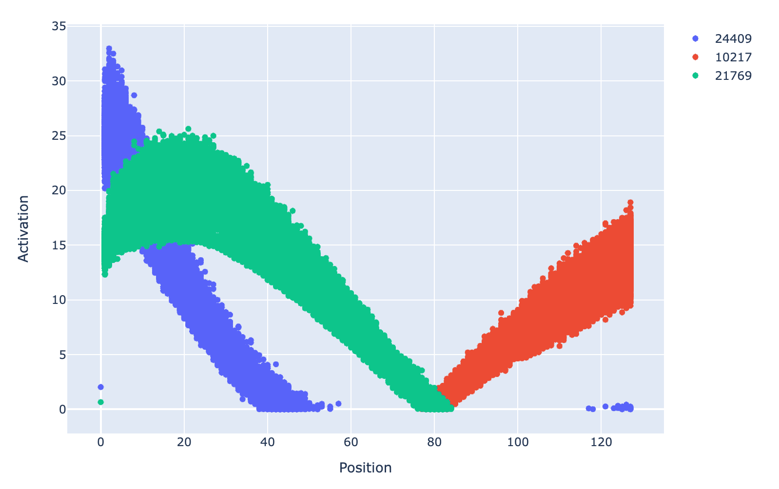
- Feature #21769 (freq: 0.627), 10217 (freq: 0.370) & 24409 (freq: 0.3372) are positional based, but possibly contain more info. The positional dependence of the activation strength for all non-zero activations is shown in the plot below for these three features. Here, the bottom 10% seem interpretable, at least the positional based info. Given the scatter in the plot, it looks like more info might be contained in the feature. Looking at max activations for a given position did not shed any further light. I don't know whether it's reasonable to expect GPT2-small to actually have & use features like this.
- Feature #21014 (freq: 0.220) fires at the 2nd position in sentences, after new lines and full stops, and then has smaller activations for 3rd, 4th & 5th position after new lines and full stops (so the bottom 10% seem interpretable, i.e. they are further away from the start of a sentence)
- Feature #16741 (freq: 0.171) unclear from the max/min activating examples, maybe polysemantic
- Feature #12123 (freq: 0.127) fires after "the", "an", "a", again stronger for the token immediately after, and weaker for 2nd, 3rd, 4th positions after. Bottom 10% seem interpretable in this context, but again there are some exceptions, so I'm not completely sure.
- Feature #22430 (freq: 0.127) fires after "," more strongly at the first position after "," and weaker for tokens at the 2nd, 3rd, 4th positions away from ",". The bottom 10% seem somewhat interpretable here, i.e. further after "," but there are exceptions so I'm not completely sure.
- Feature #6061(freq: 0.109) fires on nouns, both at high and low activations.
While I think these interpretations seem reasonable, it seems likely that some of these SAE features are at least somewhat polysemantic. They might be improved by training the SAE longer (I trained on ~300M tokens for these SAEs).
I might make dashboards or put the SAE on Neuronpedia to be able to make a better idea of these and other features.
There's also an entire literature of variations of [e.g. sparse or disentangled] autoencoders and different losses and priors that it might be worth looking at and that I suspect SAE interp people have barely explored; some of it literally decades-old. E.g. as a potential starting point https://lilianweng.github.io/posts/2018-08-12-vae/ and the citation trails to and from e.g. k-sparse autoencoders.
Interesting, thanks for sharing! Are there specific existing ideas you think would be valuable for people to look at in the context of SAEs & language models, but that they are perhaps unaware of?
This is really cool!
- I did some tests on random features for interpretability, and found them to be interpretable. However, one would need to do a detailed comparison with SAEs trained on an L1 penalty to properly understand whether this loss function impacts interpretability. For what it’s worth, the distribution of feature sparsities suggests that we should expect reasonably interpretable features.
One cheap and lazy approach is to see how many of your features have high cosine similarity with the features of an existing L1-trained SAE (e.g. "900 of the 2048 features detected by the -trained model had cosine sim > 0.9 with one of the 2048 features detected by the L1-trained model"). I'd also be interested to see individual examinations of some of the features which consistently appear across multiple training runs in the -trained model but don't appear in an L1-trained SAE on the training dataset.
Thanks!
One cheap and lazy approach is to see how many of your features have high cosine similarity with the features of an existing L1-trained SAE (e.g. "900 of the 2048 features detected by the -trained model had cosine sim > 0.9 with one of the 2048 features detected by the L1-trained model").
I looked at the cosine sims between the L1-trained reference model and one of my SAEs presented above and found:
- 2501 out of 24576 (10%) of the features detected by the -trained model had cosine sim > 0.9 with one of the 24576 features detected by the L1-trained model.
- 7774 out of 24576 (32%) had cosine sim > 0.8
- 50% have cosine sim > 0.686
I'm not sure how to interpret these. Are they low/high? They appear to be roughly similar to if I compare between two of the -trained SAEs.
I'd also be interested to see individual examinations of some of the features which consistently appear across multiple training runs in the -trained model but don't appear in an L1-trained SAE on the training dataset.
I think I'll look more at this. Some summarised examples are shown in the response above.
The other baseline would be to compare one L1-trained SAE against another L1-trained SAE -- if you see a similar approximate "1/10 have cossim > 0.9, 1/3 have cossim > 0.8, 1/2 have cossim > 0.7" pattern, that's not definitive proof that both approaches find "the same kind of features" but it would strongly suggest that, at least to me.
Summary
I experimented with alternatives to the standard L1 penalty used to promote sparsity in sparse autoencoders (SAEs). I found that including terms based on an alternative differentiable approximation of the feature sparsity in the loss function was an effective way to generate sparsity in SAEs trained on the residual stream of GPT2-small. The key findings include:
Loss functions that incorporate differentiable approximations of sparsity as an alternative to the standard L1 penalty appear to be an interesting direction for further investigation.
Motivation
Sparse autoencoders (SAEs) have been shown to be effective at extracting interpretable features from the internal activations of language models (e.g. Anthropic & Cunningham et al.). Ideally, we want SAEs to simultaneously (a) reproduce the original language model behaviour and (b) to consist of monosemantic, interpretable features. SAE loss functions usually contain two components:
The relative importance of each term is controlled by a coefficient on the L1 penalty, which allows the model to move along the trade-off between reconstruction of the language model behaviour and a highly sparse representation. In this post, I present experiments with alternatives to the standard L1 penalty to promote sparsity in SAEs.
Approximations of the sparsity
A key requirement for SAE features to be interpretable is that most of them are sparse. In this context, the sparsity, s, of a given SAE feature, f, is the fraction of tokens for which the feature has a nonzero activation. For instance, a sparsity of s=0.01 means that the feature has a nonzero post-GELU activation for 1% of all tokens. We often use the L0 norm as an average measure of sparsity over the entire SAE, defined as the average number of features with nonzero post-GELU activations per token.
In principle, we may want to simply add the value of the L0 norm to the loss function, instead of the L1 norm. However, the calculation of the L0 norm from the feature activations a, involves a function that evaluates to 0 if a = 0, otherwise to 1 for a > 0 (see blue line in Figure 1). This calculation is not differentiable and therefore it cannot be directly used in the loss function.
There are many differentiable measures of sparsity that approximate the L0 norm (Hurley & Rickard 2009). The L1 norm is one example. Another example that Anthropic recently discussed in their updates is the tanh function, that asymptotically approaches 1 for large values of the feature activation, a.
The usefulness of these approximations as a penalty for sparsity in SAE loss functions likely depends on a combination of how accurately they approximate the L0 norm, and the derivative of the measure as a function of feature activation that is used by the optimiser in the training process. To highlight this, Figure 2 shows the derivatives of the sparsity contribution with respect to the feature activation for each sparsity measure.
Figure 1 presents a further example of a sparsity measure, the function a/(a+ϵ). In this approximation, smaller values of ϵ provide a more accurate approximation of L0, while larger values of ϵ provide larger gradients for large feature activations and more moderate gradients for small feature activations. Under this approximation, the feature sparsities in a batch can be approximated as:
sf≈1nb∑bab,fab,f+ϵ
where sf is the vector of feature sparsities, nb is the batch size, ab,f are the activations for each feature and each element in the batch, and ϵ∼0.1 is a small constant. One can approximate the L0 in a similar way,
L0approx=1nb∑b∑fab,fab,f+ϵ
and include this term in the loss function as an alternative to the L1 penalty.
In addition to the loss function, recent work training SAEs on language model activations often included techniques in the training process to limit the number of dead SAE features that are produced (e.g. the resampling procedure described by Anthropic). As an attempt to limit the number of dead features that form, I experimented with adding the following term to the loss function that penalises features with a sparsity below a given threshold:
∑fRELU(log10(smin)−log10(sf))
where smin is the desired minimum sparsity threshold, and sf are the feature sparsities. Figure 3 visualises the value of this term as a function of the feature sparsity for smin=10−5.
Before this term can be directly included in the loss function, we must deal with the fact that in the expression for sf given above, the minimum sparsity it can deal with is limited by the batch size, e.g. a batch size of 4096 cannot resolve sparsities below ~0.001. To take into account arbitrarily low sparsity values, we can take the average of the sparsity of each feature over the last n training steps. We can then use this more accurate value of the sparsity in the RELU function, but with the gradients from the original expression for sf above.
In addition to the two terms presented here, I explored a wide range of alternative terms in the loss function. Many of these didn’t work, and some worked reasonably well. Some of these alternatives are discussed below.
Training the SAEs
I trained SAEs on activations of the residual stream of GPT2-small at layer 1 to have a reference point with Joseph Bloom’s models released a few weeks ago here. I initially trained a model with as similar a setup as I could to the reference model for comparison purposes, e.g. same learning rate, number of features, batch size, training steps, but I had to remove the pre-encoder bias as I found the loss function didn’t work very well with it. I checked that simply removing the pre-encoder bias from the original model setup with the L1 + ghost gradients did not generate much improvement.
I implemented the following loss function:
L=MSE+λ0L0approx+λmin∑fRELU(log10(smin)−log10(sf))
where L0approx is given by the expression above, ϵ=0.2, λmin=10−6, smin=10−5 and where I varied λ0 to vary the sparsity. I computed 5 SAEs, varying λ0 from 3×10⁻⁵ to 9×10⁻⁵. I’ll discuss the properties of these SAEs with reference to their λ0 coefficient.
The L0, MSE and number of dead features of the 5 SAEs are summarised in the following table, along with the reference model from Joseph Bloom trained with an L1 penalty (JB L1 ref). Three of the new SAEs simultaneously achieve a lower L0 and lower MSE than the reference L1 model. For instance, the λ0=5×10⁻⁵model has a value of L0 that is 6% lower and a MSE that is 30% lower than the reference L1 model. This seems promising and worth exploring further.
Figure 4 shows the evolution of L0 and the mean-squared error during the training process for these 5 SAEs trained on the above loss function. We can see that they reach a better region of the parameter space in terms of L0 and the mean squared error, as compared to the reference L1 model.
Feature sparsity distributions
A useful metric to look at when training SAEs is the distribution of feature sparsities. Plotting these distributions can reveal artefacts or inefficiencies in the training process, such as large numbers of features with low sparsity (or dead features), large numbers of high density features, and the shape of the overall distribution of sparsities. Figure 5 shows the feature sparsities for the five new SAEs models trained on the loss function described above, compared to the reference L1 model. The distributions of the 5 new models are slightly wider than the reference L1 model. We can also see the significant number of dead features (i.e. at a log sparsity of -10) in the reference L1 model compared to the new models. The light grey vertical line at a log sparsity of -5 indicates the value of smin, the sparsity threshold below which features are penalised in the loss function. We can see that there is a sharp drop-off in features just above and at this threshold. This suggests that the loss function term to discourage the formation of highly sparse features is working as intended.
Figure 6 shows the same distribution for the λ0=7×10⁻⁵ model and the L1 reference model on a log-scale. Here we see more significant differences between the feature distributions at higher sparsities. The λ0=7×10⁻⁵ model is closer to a power law distribution compared to the L1 reference model, which contains a bump at around -2. This is reminiscent of Zipf’s law for the frequency of words in natural language. Since we are training on the residual stream before layer 1 of GPT2-small, it would not be surprising if the distribution of features closely reflected the distribution of words in natural language. However, this is just speculation and requires proper investigation. A quick comparison shows the distribution matches a power law with slope around -0.9, although there appears to still be a small bump in the feature sparsity distribution around a log sparsity of -2. This bump may be reflective of the reality of the feature distribution in GPT2-small, or may be an artefact of the imperfect training process.
High density features
The λ0=7×10⁻⁵ model contains a small number (7) of high density features with sparsities above 0.2 that the reference L1 model does not contain. A quick inspection of the max activating tokens of these features suggests they are reasonably interpretable. Several appeared to be positional based features. For instance, one fired strongly on tokens at positions 1, 2 & 3, and weaker for later positions. Another fired strongly at position 127 (the final token in each context) and weaker for earlier positions. One was firing on short prepositions such as “on”, “at”. Another was firing strongly shortly after new line tokens. In principle, these features can be made more sparse, if desired for interpretability purposes, but it’s not clear whether that’s needed, desired, or what the cost associated with enforcing this would be. Interestingly, the same or very similar features are present in all models from λ0=3×10⁻⁵ to λ0=9×10⁻⁵.
Avoiding dead features
Dead features are a significant problem in the training of SAEs. Whatever procedure is used to promote sparsity also runs the risk of generating dead features that can no longer be useful in the SAE. Methods like re-sampling and ghost gradients have been proposed to try to improve this situation.
The third term in the loss function written above helps to avoid the production of dead features. As a result, dead features can be greatly inhibited or almost completely eliminated in these new SAEs. The light grey vertical line in the figure indicates the value of smin=10−5, the sparsity threshold below which features are penalised in the loss function. Note the sharp drop-off in feature sparsity below 10−5. Further experimentation with hyperparameters may reduce the number of dead features to ~0, although it’s possible that this comes at some cost to the rest of the model.
The behaviour of the RELU term in the loss function depends somewhat on the learning rate. A lower learning rate tends to nudge features back to the desired sparsity range, shortly after the sparsity drops outside the desired range. A large learning rate can either cause oscillations (for over-dense features) or can cause over-sparse features to be bumped back to high density features, almost as if they are resampled.
Comparison of training curves
Evolution of mean squared error & L0
Figures 7 & 8 show the evolution of the MSE and L0 during the training process. The L0 and MSE trained on L0approx follow a slightly different evolution to the L1 reference model. In addition, the L0 and MSE are still noticeably declining after training on 80k steps (~300M tokens), as compared to the reference L1 model that seems to flatten out beyond a given time-step in the training process. This suggests that training on more tokens may improve the SAEs.
Evolution of L1
Figure 9 compares the L1 norms of the new models with the L1 reference model. The fact that the L1 norms of the new models are substantially different to the model with the L1 penalty (and note that W_dec is normalised in all models) is evidence that the SAEs are different. This is obviously not related to which SAE is better, only that they are different.
Discussion
Advantages of this loss function
Shortcomings and other considerations
Alternative loss terms based on the sparsity
Given an approximation of the sparsity distribution in the loss function, there are many different terms that one could construct to add to the loss function. Some examples include:
I explored these terms and found that they all worked to varying extents. Ultimately, they were not more effective than the function I chose to discuss in detail above. Further investigation will probably uncover better loss function terms, or a similar function, but based on a better approximation of the feature sparsity.
Summary of other architecture and hyperparameter tests
Acknowledgements
I'd like to thank Evan Anders, Philip Quirke, Joseph Bloom and Neel Nanda for helpful discussion and feedback. This work was supported by a grant from Open Philanthropy.
MSE computed by Joseph’s old definition for comparison purposes