Hey Joseph (and coauthors),
Your directions are really fantastic. I hope you don't mind, but I generated the activation data for the first 3000+ directions for each of the 12 layers and uploaded your directions to Neuronpedia:
https://www.neuronpedia.org/gpt2-small/res-jb
Your directions are also linked on the home page and the model page.
They're also accessible by layer (sorted by top activation), eg layer 6: https://neuronpedia.org/gpt2-small/6-res-jb
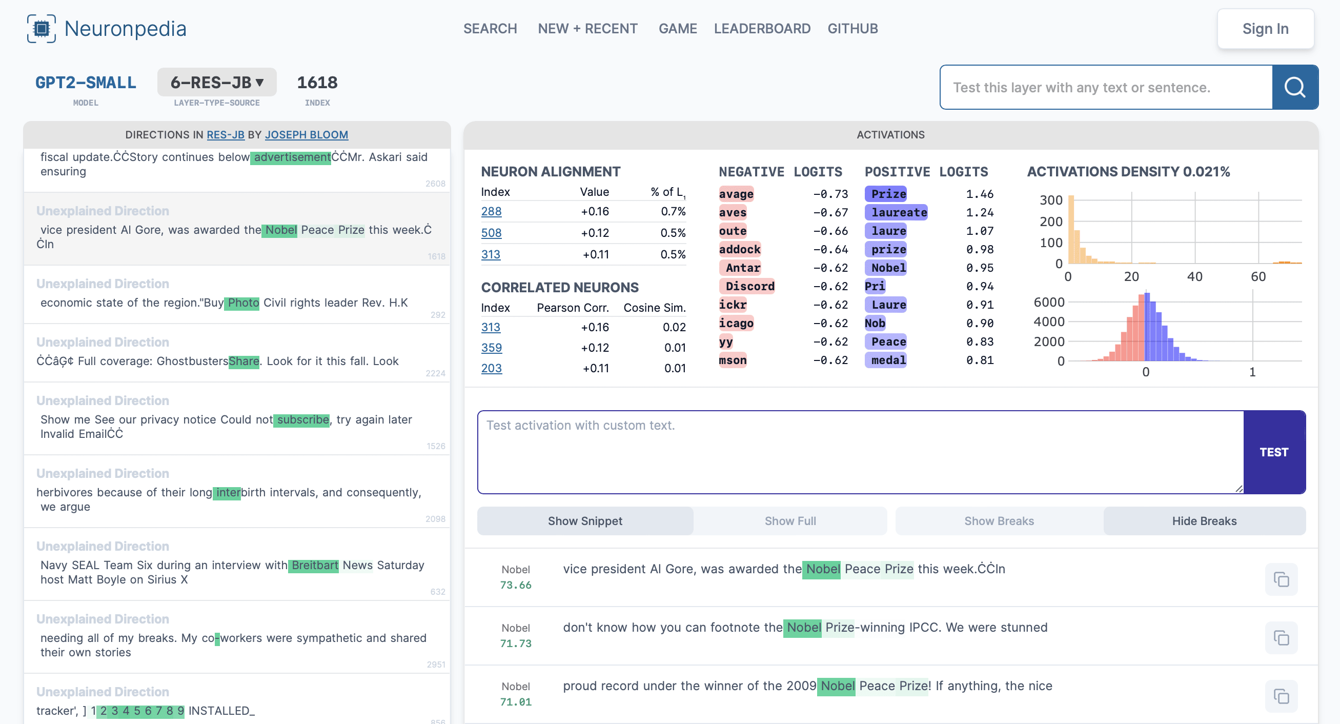
I added the "Anthropic dashboard" to Neuronpedia for your dataset.
Explanations, comments, and autointerp scoring are also working - anyone can do this:
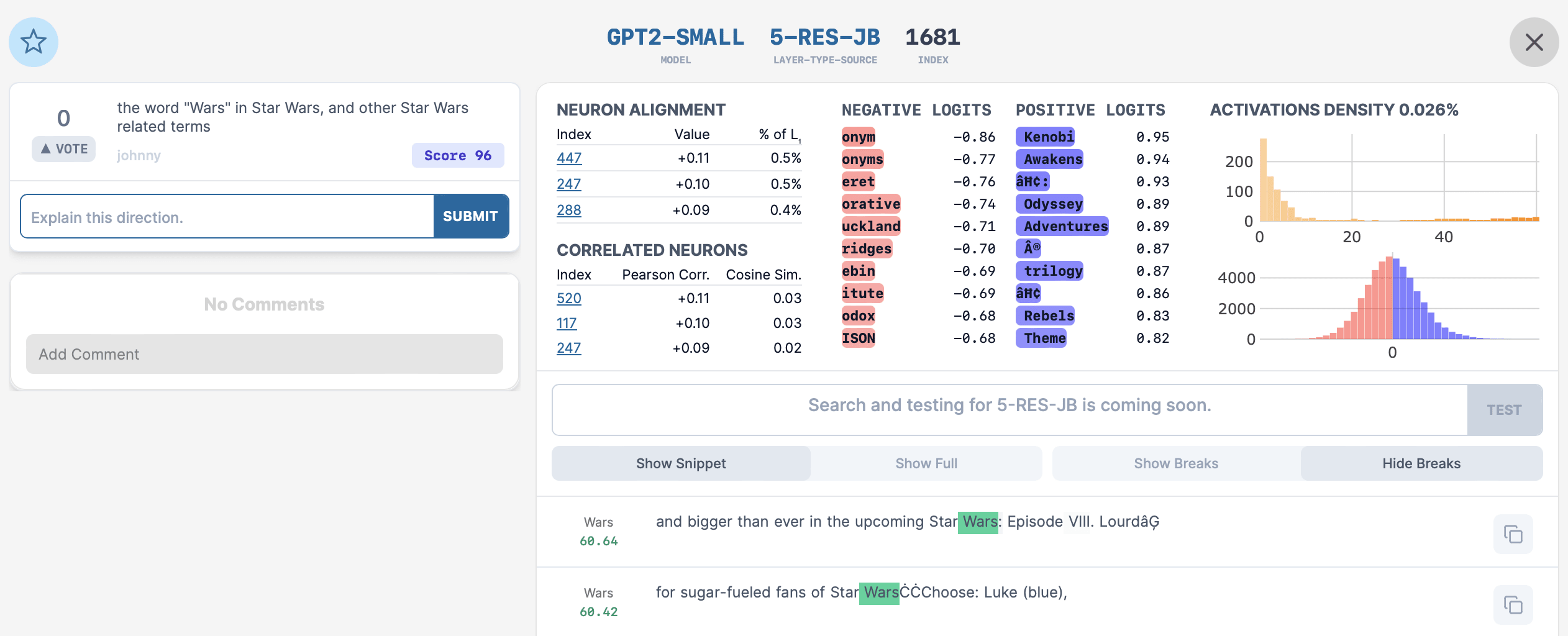
- Click a direction and submit explanation on the top-left. Here's another Star Wars direction (5-RES-JB:1681) where GPT4 gave me a score of 96:
- Click the score for the scoring details:
- Click the score for the scoring details:

I plan to do some autointerp explaining on a batch of these directions too.
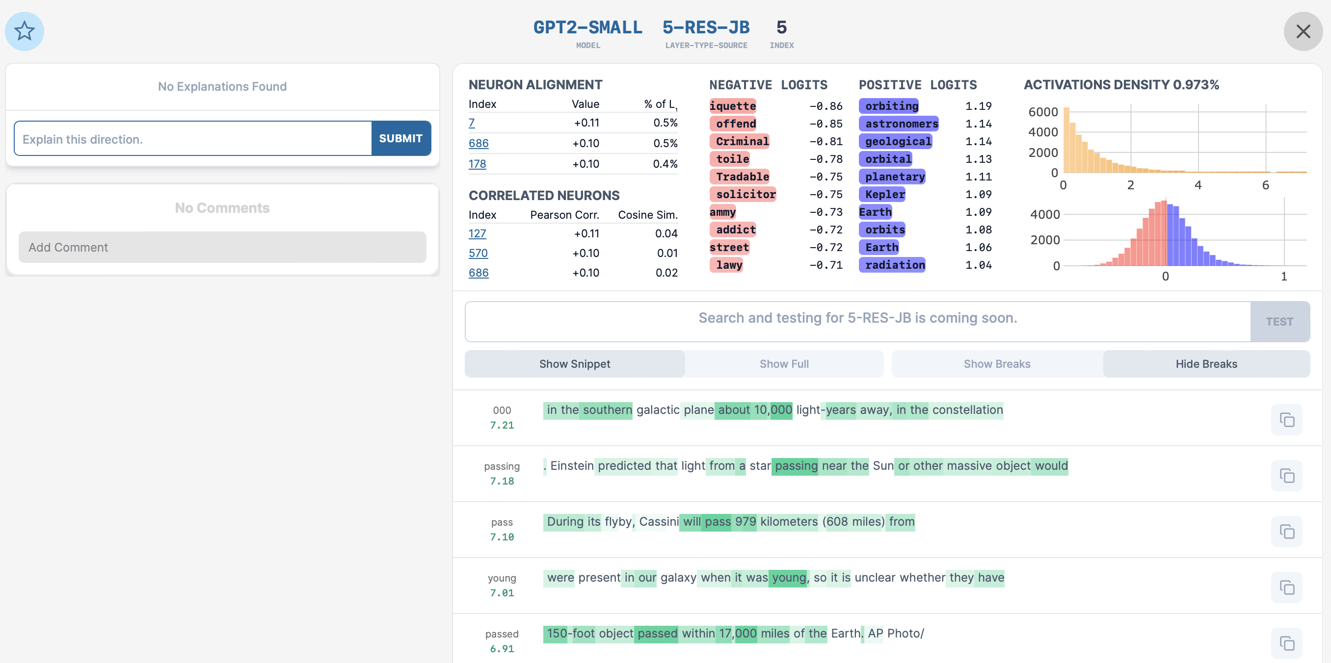
Btw - your directions are so good that it's easy to find super interesting stuff. 5-RES-JB:5 is about astronomy:
I'm aware that you're going to do some library updates to get even better directions, and I'm excited for that - will re-generate/upload all layers after the new changes come in.
Things that I'm still working on and hope to get working in the next few days:
- Making activation testing work for each neuron
- "Search / test" the same way that we have search/test for OpenAI's directions
Again, your directions look fantastic - congrats. I hope this is useful/interesting for you and anyone trying to browse/explain them. Also, I didn't know how to provide a citation/reference to you (and your team?) so I just used RES-JB = Residuals by Joseph Bloom and included links to all relevant sources on your directions page.
If there's anything you'd like me to modify about this, or any feature you'd like me to add to make it better, please do not hesitate to let me know.
Thanks for doing this, I'm excited about Neuronpedia focusing on SAE features! I expect this to go much better than neuron interpretability
Our reconstruction scores were pretty good. We found GPT2 small achieves a cross entropy loss of about 3.3, and with reconstructed activations in place of the original activation, the CE Log Loss stays below 3.6.
Unless my memory is screwing up the scale here, 0.3 CE Loss increase seems quite substantial? A 0.3 CE loss increase on the pile is roughly the difference between Pythia 410M and Pythia 2.8B. And do I see it right that this is the CE increase maximum for adding in one SAE, rather than all of them at the same time? So unless there is some very kind correlation in these errors where every SAE is failing to reconstruct roughly the same variance, and that variance at early layers is not used to compute the variance SAEs at later layers are capturing, the errors would add up? Possibly even worse than linearly? What CE loss do you get then?
Have you tried talking to the patched models a bit and compared to what the original model sounds like? Any discernible systematic differences in where that CE increase is changing the answers?
> 0.3 CE Loss increase seems quite substantial? A 0.3 CE loss increase on the pile is roughly the difference between Pythia 410M and Pythia 2.8B
My personal guess is that something like this is probably true. However since we're comparing OpenWebText and the Pile and different tokenizers, we can't really compare the two loss numbers, and further there is not GPT-2 extra small model so currently we can't compare these SAEs to smaller models. But yeah in future we will probably compare GPT-2 Medium and GPT-2 Large with SAEs attached to the smaller models in the same family, and there will probably be similar degradation at least until we have more SAE advances.
One experiment here is to see if specific datapoints that have worse CE-diff correlate across layers. Last time I did a similar experiment, I saw a very long tail of datapoints that were worse off (for just one layer of gpt2-small), but the majority of datapoints had similar CE. So Joseph's suggested before to UMAP these datapoints & color by their CE-diff (or other methods to see if you could separate out these datapoints).
If someone were to run this experiment, I'd also be interested if you removed the k-lowest features per datapoint, checking the new CE & MSE. In the SAE-work, the lowest activating features usually don't make sense for the datapoint. This is to test the hypothesis:
- Low-activating features are noise or some acceptable false alarm rate true to the LLM2. (ie SAE's capture what we care about)
- Actually they're important for CE in ways we don't understand. (ie SAE's let in un-interpretable feature activations which are important, but?)
For example, if you saw better CE-diff when removing low-activating features, up to a specific k, then SAE's are looking good!
Neel and I recently tried to interpret a language model circuit by attaching SAEs to the model. We found that using an L0=50 SAE while only keeping the top 10 features by activation value per prompt (and zero ablating the others) was better than an L0=10 SAE by our task-specific metric, and subjective interpretability. I can check how far this generalizes.
I'd be excited about reading about / or doing these kinds of experiments. My weak prediction is that low activating features are important in specific examples where nuance matters and that what we want is something like an "adversarially robust SAE" which might only be feasible with current SAE methods on a very narrow distribution.
A mini experiment I did which motivates this: I did an experiment with an SAE at the residual stream where I looked at the attention pattern of an attention head immediately following the head as function of k, where we take the top-k SAE features in the reconstruction. I found that if the head was attending to "Mary" in the original forward pass (and not "John"), then a k of 3 was good enough to have it attend to Mary and not John. But if I replaced John with Martha, the minimum k such that the head attended to Mary increased.
There's a few things to note. Later layers have:
- worse CE-diff & variance explained (e.g. the layer 0 CE-diff seems great!)
- larger L2 norms in the original LLM activations
- worse ratio of reconstruction-L2/original-L2 (meaning it's under-normed)*
- less dead features (maybe they need more features?)
For (3), we might expect under-normed reconstructions because there's a trade-off between L1 & MSE. After training, however, we can freeze the encoder, locking in the L0, and train on the decoder or scalar multiples of the hidden layer (h/t to Ben Wright for first figuring this out).
(4) Seems like a pretty easy experiment to try to just vary num of features to see if this explains part of the gap.
*
Unless my memory is screwing up the scale here, 0.3 CE Loss increase seems quite substantial? A 0.3 CE loss increase on the pile is roughly the difference between Pythia 410M and Pythia 2.8B.
Thanks for raising this! I had wanted to find a comparison in terms of different model performances to help me quantify this so I'm glad to have this as a reference.
And do I see it right that this is the CE increase maximum for adding in one SAE, rather than all of them at the same time? So unless there is some very kind correlation in these errors where every SAE is failing to reconstruct roughly the same variance, and that variance at early layers is not used to compute the variance SAEs at later layers are capturing, the errors would add up? Possibly even worse than linearly? What CE loss do you get then?
Have you tried talking to the patched models a bit and compared to what the original model sounds like? Any discernible systematic differences in where that CE increase is changing the answers?
While I have explored model performance with SAEs at different layers, I haven't done so with more than one SAE or explored sampling from the model with the SAE. I've been curious about systematic errors induced by the SAE but a few brief experiments with earlier SAEs/smaller models didn't reveal any obvious patterns. I have once or twice looked at the divergence in the activations after an SAE has been added and found that errors in earlier layers propagated.
One thought I have on this is that if we take the analogy to DNA sequencing seriously, relatively minor errors in DNA sequencing make the resulting sequences useless. If you get one or two base pairs wrong then try to make bacteria express the printed gene (based on your sequencing) then you'll kill that bacteria. This gives me the intuition that I absolutely expect we could have fairly accurate measurements with some error and that the resulting error is large.
To bring it back to what I suspect is the main point here: We should amend the statement to say "Our reconstruction scores were pretty good as compared to our previous results".
It bothers me quite a bit that SAEs don't recover performance better, but I think this is a fairly well defined and that the community can iterate on both via improvements to SAEs and looking for nearby alternatives. For example, I'm quite excited to experiment with any alternative architectures/training procedures that come out of the theory of computation in superposition line of work.
One productive direction inspired by thinking of this as sequencing is that we should have lots of SAEs trained on the same model and show that they get very similar results (to give us more confidence we have a better estimate of the true underlying features). It's standard in DNA/RNA/Protein sequencing to run methods many times over. I think once we see evidence that we get good results along those lines, we should be more interested in / raise our standards for model performance with reconstructed SAEs.
Is the drop of eval loss when attaching SAEs a crux for the SAE research direction to you? I agree it's not ideal, but to me the comparison of eval loss to smaller models only makes sense if the goal of the SAE direction is making a full-distribution competitive model. Explaining narrow tasks, or just using SAEs for monitoring/steering/lie detection/etc. doesn't require competitive eval loss. (Note that I have varying excitement about all these goals, e.g. some pessimism about steering)
If the SAEs are not full-distribution competitive, I don't really trust that the features they're seeing are actually the variables being computed on in the sense of reflecting the true mechanistic structure of the learned network algorithm and that the explanations they offer are correct[1]. If I pick a small enough sub-distribution, I can pretty much always get perfect reconstruction no matter what kind of probe I use, because e.g. measured over a single token the network layers will have representation rank , and the entire network can be written as a rank- linear transform. So I can declare the activation vector at layer to be the active "feature", use the single entry linear maps between SAEs to "explain" how features between layers map to each other, and be done. Those explanations will of course be nonsense and not at all extrapolate out of distributon. I can't use them to make a causal model that accurately reproduces the network's behavior or some aspect of it when dealing with a new prompt.
We don't train SAEs on literally single tokens, but I would be worried about the qualitative problem persisting. The network itself doesn't have a million different algorithms to perform a million different narrow subtasks. It has a finite description length. It's got to be using a smaller set of general algorithms that handle all of these different subtasks, at least to some extent. Likely more so for more powerful and general networks. If our "explanations" of the network then model it in terms of different sets of features and circuits for different narrow subtasks that don't fit together coherently to give a single good reconstruction loss over the whole distribution, that seems like a sign that our SAE layer activations didn't actually capture the general algorithms in the network. Thus, predictions about network behaviour made on the basis of inspecting causal relationships between these SAE activations might not be at all reliable, especially predictions about behaviours like instrumental deception which might be very mechanistically related to how the network does well on cross-domain generalisation.
- ^
As in, that seems like a minimum requirement for the SAEs to fulfil. Not that this would be to make me trust predictions about generalisation based on stories about SAE activations.
(This reply is less important than my other)
> The network itself doesn't have a million different algorithms to perform a million different narrow subtasks
For what it's worth, this sort of thinking is really not obvious to me at all. It seems very plausible that frontier models only have their amazing capabilities through the aggregation of a huge number of dumb heuristics (as an aside, I think if true this is net positive for alignment). This is consistent with findings that e.g. grokking and phase changes are much less common in LLMs than toy models.
(Two objections to these claims are that plausibly current frontier models are importantly limited, and also that it's really hard to prove either me or you correct on this point since it's all hand-wavy)
Thanks for the first sentence -- I appreciate clearly stating a position.
measured over a single token the network layers will have representation rank 1
I don't follow this. Are you saying that the residual stream at position 0 in a transformer is a function of the first token only, or something like this?
If so, I agree -- but I don't see how this applies to much SAE[1] or mech interp[2] work. Where do we disagree?
- ^
E.g. in this post here we show in detail how an "inside a question beginning with which" SAE feature is computed from which and predicts question marks (I helped with this project but didn't personally find this feature)
- ^
More generally, in narrow distribution mech interp work such as the IOI paper, I don't think it makes sense to reduce the explanation to single-token perfect accuracy probes since our explanation generalises fairly well (e.g. the "Adversarial examples" in Section 4.4 Alexandre found, for example)
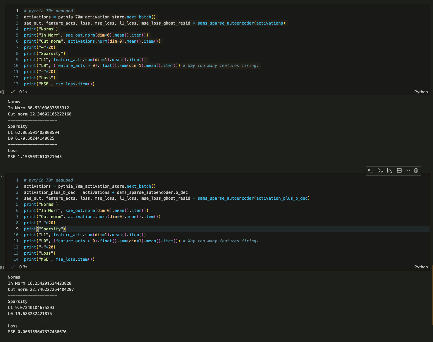
I tried replicating your statistics using my own evaluation code (in evaluation.py here). I pseudo-randomly chose layer 1 and layer 7. Sadly, my results look rather different from yours:
| Layer | MSE Loss | % Variance Explained | L1 | L0 | % Alive | CE Reconstructed |
|---|---|---|---|---|---|---|
| 1 | 0.11 | 92 | 44 | 17.5 | 54 | 5.95 |
| 7 | 1.1 | 82 | 137 | 65.4 | 95 | 4.29 |
Places where our metrics agree: L1 and L0.
Places where our metrics disagree, but probably for a relatively benign reason:
- Percent variance explained: my numbers are slightly lower than yours, and from a brief skim of your code I think it's because you're calculating variance slightly incorrectly: you're not subtracting off the activation's mean before doing .pow(2).sum(-1). This will slightly overestimate the variance of the original activations, so probably also overestimate percent variance explained.
- Percent alive: my numbers are slightly lower than yours, and this is probably because I determined whether neurons are alive on a (somewhat small) batch of 8192 tokens. So my number is probably an underestimate and yours is correct.
Our metrics disagree strongly on CE reconstructed, and this is a bit alarming. It means that either you have a bug which significantly underestimates reconstructed CE loss, or I have a bug which significantly overestimates it. I think I'm 50/50 on which it is. Note that according to my stats, your MSE loss is kinda bad, which would suggest that you should also have high CE reconstructed (especially when working with residual stream dictionaries! (in contrast to e.g. MLP dictionaries which are much more forgiving)).
Spitballing a possible cause: when computing CE loss, did you exclude padding tokens? If not, then it's possible that many of the tokens on which you're computing CE are padding tokens, which is artificially making your CE look extremely good.
Here is my code. You'll need to pip install nnsight before running it. Many thanks to Caden Juang for implementing the UnifiedTransformer functionality in nnsight, which is a crazy Frankenstein marriage of nnsight and transformer_lens; it would have been very hard for me to attempt this replication without this feature.
Oh no. I'll look into this and get back to you shortly. One obvious candidate is that I was reporting CE for some batch at the end of training that was very small and so the statistics likely had high variance and the last datapoint may have been fairly low. In retrospect I should have explicitly recalculated this again post training. However, I'll take a deeper dive now to see what's up.
I've run some of the SAE's through more thorough eval code this morning (getting variance explained with the centring and calculating mean CE losses with more batches). As far as I can tell the CE loss is not that high at all and the MSE loss is quite low. I'm wondering whether you might be using the wrong hooks? These are resid_pre so layer 0 is just the embeddings and layer 1 is after the first transformer block and so on. One other possibility is that you are using a different dataset? I trained these SAEs on OpenWebText. I don't much padding at all, that might be a big difference too. I'm curious to get to the bottom of this.
One sanity check I've done is just sampling from the model when using the SAE to reconstruct activations and it seems to be about as good, which I think rules out CE loss in the ranges you quote above.
For percent alive neurons a batch size of 8192 would be far too few to estimate dead neurons (since many neurons have a feature sparsity < 10**-3.
You're absolutely right about missing the centreing in percent variance explained. I've estimated variance explained again for the same layers and get very similar results to what I had originally. I'll make some updates to my code to produce CE score metrics that have less variance in the future at the cost of slightly more train time.
If we don't find a simple answer I'm happy to run some more experiments but I'd guess an 80% probability that there's a simple bug which would explain the difference in what you get. Rank order of most likely: Using the wrong activations, using datapoints with lots of padding, using a different dataset (I tried the pile and it wasn't that bad either).
In the notebook I link in my original comment, I check that the activations I get out of nnsight are the same as the activations that come from transformer_lens. Together with the fact that our sparsity statistics broadly align, I'm guessing that the issue isn't that I'm extracting different activations than you are.
Repeating my replication attempt with data from OpenWebText, I get this:
| Layer | MSE Loss | % Variance Explained | L1 | L0 | % Alive | CE Reconstructed |
|---|---|---|---|---|---|---|
| 1 | 0.069 | 95 | 40 | 15 | 46 | 6.45 |
| 7 | 0.81 | 86 | 125 | 59.2 | 96 | 4.38 |
Broadly speaking, same story as above, except that the MSE losses look better (still not great), and that the CE reconstructed looks very bad for layer 1.
I don't much padding at all, that might be a big difference too.
Seems like there was a typo here -- what do you mean?
Logan Riggs reports that he tried to replicate your results and got something more similar to you. I think Logan is making decisions about padding and tokenization more like the decisions you make, so it's possible that the difference is down to something around padding and tokenization.
Possible next steps:
- Can you report your MSE Losses (instead of just variance explained)?
- Can you try to evaluate the residual stream dictionaries in the 5_32768 set released here? If you get CE reconstructed much better than mine, then it means that we're computing CE reconstructed in different ways, where your way consistently reports better numbers. If you get CE reconstructed much worse than mine, then it might mean that there's a translation error between our codebases (e.g. using different activations).
Another sanity check: when you compute CE loss using the same code that you use when computing CE loss when activations are reconstructed by the autoencoders, but instead of actually using the autoencoder you just plug the correct activations back in, do you get the same answer (~3.3) as when you evaluate CE loss normally?
- MSE Losses were in the WandB report (screenshot below).
- I've loaded in your weights for one SAE and I get very bad performance (high L0, high L1, and bad MSE Loss) at first.
- It turns out that this is because my forward pass uses a tied decoder bias which is subtracted from the initial activations and added as part of the decoder forward pass. AFAICT, you don't do this.
- To verify this, I added the decoder bias to the activations of your SAE prior to running a forward pass with my code (to effectively remove the decoder bias subtraction from my method) and got reasonable results.
- I've screenshotted the Towards Monosemanticity results which describes the tied decoder bias below as well.
I'd be pretty interested in knowing if my SAEs seem good now based on your evals :) Hopefully this was the only issue.
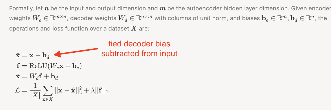
My SAEs also have a tied decoder bias which is subtracted from the original activations. Here's the relevant code in dictionary.py
def encode(self, x):
        return nn.ReLU()(self.encoder(x - self.bias))

    def decode(self, f):
        return self.decoder(f) + self.bias

    def forward(self, x, output_features=False, ghost_mask=None):
            [...]
            f = self.encode(x)
            x_hat = self.decode(f)
            [...]
            return x_hat
Note that I checked that our SAEs have the same input-output behavior in my linked colab notebook. I think I'm a bit confused why subtracting off the decoder bias had to be done explicitly in your code -- maybe you used dictionary.encoder and dictionary.decoder instead of dictionary.encode and dictionary.decode? (Sorry, I know this is confusing.) ETA: Simple things I tried based on the hypothesis "one of us needs to shift our inputs by +/- the decoder bias" only made things worse, so I'm pretty sure that you had just initially converted my dictionaries into your infrastructure in a way that messed up the initial decoder bias, and therefore had to hand-correct it.
I note that the MSE Loss you reported for my dictionary actually is noticeably better than any of the MSE losses I reported for my residual stream dictionaries! Which layer was this? Seems like something to dig into.
Ahhh I see. Sorry I was way too hasty to jump at this as the explanation. Your code does use the tied decoder bias (and yeah, it was a little harder to read because of how your module is structured). It is strange how assuming that bug seemed to help on some of the SAEs but I ran my evals over all your residual stream SAE's and it only worked for some / not others and certainly didn't seem like a good explanation after I'd run it on more than one.
I've been talking to Logan Riggs who says he was able to load in my SAEs and saw fairly similar reconstruction performance to to me but that outside of the context length of 128 tokens, performance markedly decreases. He also mentioned your eval code uses very long prompts whereas mine limits to 128 tokens so this may be the main cause of the difference. Logan mentioned you had discussed this with him so I'm guessing you've got more details on this than I have? I'll build some evals specifically to look at this in the future I think.
Scientifically, I am fairly surprised about the token length effect and want to try training on activations from much longer context sizes now. I have noticed (anecdotally) that the number of features I get sometimes increases over the prompt so an SAE trained on activations from shorter prompts are plausibly going to have a much easier time balancing reconstruction and sparsity, which might explain the generally lower MSE / higher reconstruction. Though we shouldn't really compare between models and with different levels of sparsity as we're likely to be at different locations on the pareto frontier.
One final note is that I'm excited to see whether performance on the first 128 tokens actually improves in SAEs trained on activations from > 128 token forward passes (since maybe the SAE becomes better in general).
Yep, as you say, @Logan Riggs figured out what's going on here: you evaluated your reconstruction loss on contexts of length 128, whereas I evaluated on contexts of arbitrary length. When I restrict to context length 128, I'm able to replicate your results.
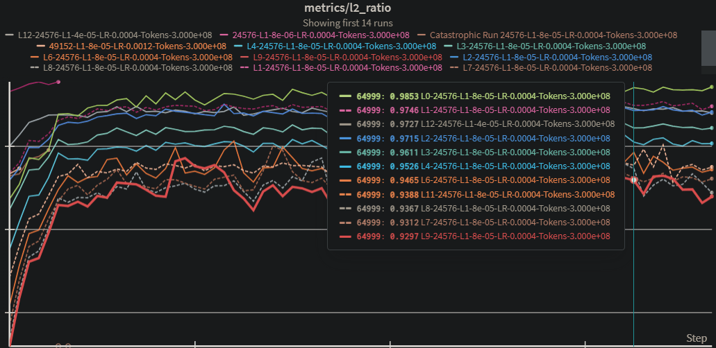
Here's Logan's plot for one of your dictionaries (not sure which)
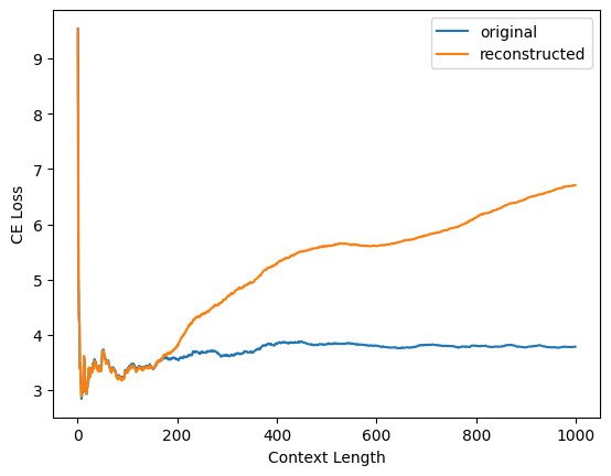
and here's my replication of Logan's plot for your layer 1 dictionary
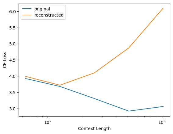
Interestingly, this does not happen for my dictionaries! Here's the same plot but for my layer 1 residual stream output dictionary for pythia-70m-deduped

(Note that all three plots have a different y-axis scale.)
Why the difference? I'm not really sure. Two guesses:
- The model: GPT2-small uses learned positional embeddings whereas Pythia models use rotary embeddings
- The training: I train my autoencoders on variable-length sequences up to length 128; left padding is used to pad shorter sequences up to length 128. Maybe this makes a difference somehow.
In terms of standardization of which metrics to report, I'm torn. On one hand, for the task your dictionaries were trained on (reconstruction activations taken from length 128 sequences), they're performing well and this should be reflected in the metrics. On the other hand, people should be aware that if they just plug your autoencoders into GPT2-small and start doing inference on inputs found in the wild, things will go off the rails pretty quickly. Maybe the answer is that CE diff should be reported both for sequences of the same length used in training and for arbitrary-length sequences?
The fact that Pythia generalizes to longer sequences but GPT-2 doesn't isn't very surprising to me -- getting long context generalization to work is a key motivation for rotary, e.g. the original paper https://arxiv.org/abs/2104.09864
This comment is about why we were getting different MSE numbers. The answer is (mostly) benign -- a matter of different scale factors. My parallel comment, which discusses why we were getting different CE diff numbers is the more important one.
When you compute MSE loss between some activations and their reconstruction , you divide by variance of , as estimated from the data in a batch. I'll note that this doesn't seem like a great choice to me. Looking at the resulting training loss:
where is the encoding of by the autoencoder and is the L1 regularization constant, we see that if you scale by some constant , this will have no effect on the first term, but will scale the second term by . So if activations generically become larger in later layers, this will mean that the sparsity term becomes automatically more strongly weighted.
I think a more principled choice would be something like
where we're no longer normalizing by the variance, and are also using sqrt(MSE) instead of MSE. (This is what the dictionary_learning repo does.) When you scale by a constant , this entire expression scales by a factor of , so that the balance between reconstruction and sparsity remains the same. (On the other hand, this will mean that you might need to scale the learning rate by , so perhaps it would be reasonable to divide through this expression by ? I'm not sure.)
Also, one other thing I noticed: something which we both did was to compute MSE by taking the mean over the squared difference over the batch dimension and the activation dimension. But this isn't quite what MSE usually means; really we should be summing over the activation dimension and taking the mean over the batch dimension. That means that both of our MSEs are erroneously divided by a factor of the hidden dimension (768 for you and 512 for me).
This constant factor isn't a huge deal, but it does mean that:
- The MSE losses that we're reporting are deceptively low, at least for the usual interpretation of "mean squared error"
- If we decide to fix this, we'll need to both scale up our L1 regularization penalty by a factor of the hidden dimension (and maybe also scale down the learning rate).
This is a good lesson on how MSE isn't naturally easy to interpret and we should maybe just be reporting percent variance explained. But if we are going to report MSE (which I have been), I think we should probably report it according to the usual definition.
- We store activations in a buffer of ~500k tokens which is refilled and shuffled whenever 50% of the tokens are used (ie: Neel’s approach).
I am not sure I understand the reasoning around this approach. Why do you want to refill and shuffle tokens whenever 50% of the tokens are used? Is this just tokens in the training set or also the test set? In Neel's code I didn't see a train/test split, isn't that important? Also, can you track the number of epochs of training when using this buffer method (it seems like that makes it more difficult)?
Why do you want to refill and shuffle tokens whenever 50% of the tokens are used?
Neel was advised by the authors that it was important minimise batches having tokens from the same prompt. This approach leads to a buffer having activations from many different prompts fairly quickly.
Is this just tokens in the training set or also the test set? In Neel's code I didn't see a train/test split, isn't that important?
I never do evaluations on tokens from prompts used in training, rather, I just sample new prompts from the buffer. Some library set aside a set of tokens to do evaluations on which are re-used. I don't currently do anything like this but it might be reasonable. In general, I'm not worried about overfitting.
Also, can you track the number of epochs of training when using this buffer method (it seems like that makes it more difficult)?
Epochs in training makes sense in a data-limited regime which we aren't in. OpenWebText has way more tokens than we ever train any sparse autoencoder on so we're always on way less than 1 epoch. We never reuse the same activations when training, but may use more than one activation from the same prompt.
Neel was advised by the authors that it was important minimise batches having tokens from the same prompt. This approach leads to a buffer having activations from many different prompts fairly quickly.
Oh I see, it's a constraint on the tokens from the vocabulary rather than the prompts. Does the buffer ever reuse prompts or does it always use new ones?
Why do you scale your MSE by 1/(x_centred**2).sum(dim=-1, keepdim=True).sqrt() ? In particular, I'm confused about why you have the square root. Shouldn't it just be 1/(x_centred**2).sum(dim=-1, keepdim=True)?
24, 576 prompts of length 128 = 3, 145, 728.
With features that fire less frequently this won't be enough, but for these we seemed to find some activations (if not highly activating) for all features.
For the dashboards, did you filter out the features that fire less frequently? I looked through a few and didn't notice any super low density ones.
On wandb, the dashboards were randomly sampled but we've since uploaded all features to Neuronpedia https://www.neuronpedia.org/gpt2-small/res-jb. The log sparsity is stored in the huggingface repo so you can look for the most sparse features and check if their dashboards are empty or not (anecdotally most dashboards seem good, beside the dead neurons in the first 4 layers).
Browse these SAE Features on Neuronpedia!
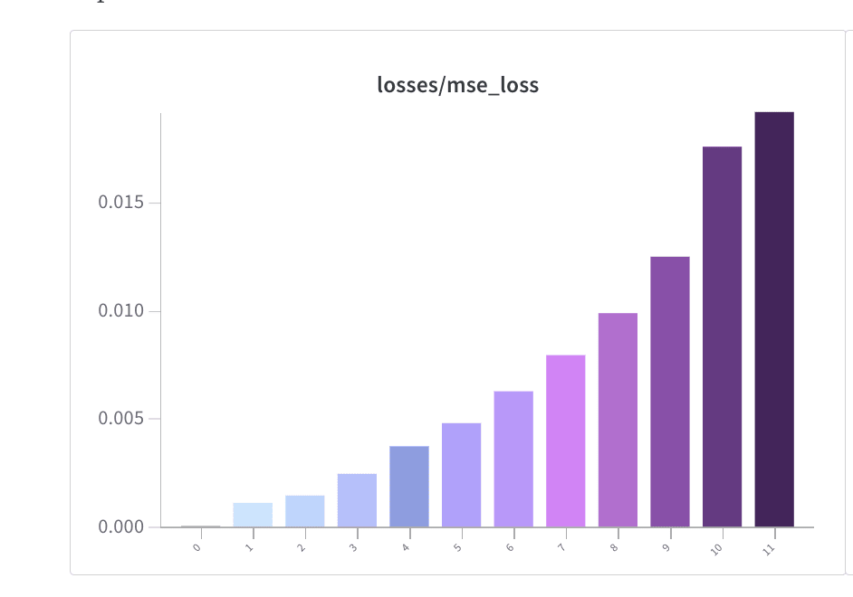
Update 1: Since we posted this last night, someone pointed out that our implementation of ghost grads has a non-trivial error (which makes the results a-priori quite surprising). We computed the ghost grad forward pass using Exp(Relu(W_enc(x)[dead_neuron_mask])) rather than Exp((W_enc(x)[dead_neuron_mask])). I'm running some ablation experiments now to get to the bottom of this.
Update 2: I've since investigated this further and run some ablation studies with the following results. Ghost grads weren't working as intended due to the Exp(Relu(x)) bug but the resulting SAE's were still quite good (later layers had few dead neurons simply because when we dropped the number of features, you get less dead neurons. I've found that with a correct ghost grads implementation, you can get less dead neurons and will update the library shortly. (I will make edits to the rest of this post to reflect my current views). Sorry for the confusion.
This work was produced as part of the ML Alignment & Theory Scholars Program - Winter 2023-24 Cohort, under mentorship from Neel Nanda and Arthur Conmy. Funding for this work was provided by the Manifund Regranting Program and donors as well as LightSpeed Grants.
This is intended to be a fairly informal post sharing a set of Sparse Autoencoders trained on the residual stream of GPT2-small which achieve fairly good reconstruction performance and contain fairly sparse / interpretable features. More importantly, advice from Anthropic and community members has enabled us to train these fairly more efficiently / faster than before. The specific methods that were most useful were: ghost gradients, learning rate warmup, and initializing the decoder bias with the geometric median. We discuss each of these in more detail below.
5 Minute Summary
We’re publishing a set of 12 Sparse AutoEncoders for the GPT2 Small residual stream.
Readers can access the Sparse Autoencoder weights in this HuggingFace Repo. Training code and code for loading the weights / model and data loaders can be found in this Github Repository. Training curves and feature dashboards can also be found in this wandb report. Users can download all 25k feature dashboards generated for layer 2 and 10 SAEs and the first 5000 of the layer 5 SAE features here (note the left hand of column of the dashboards should currently be ignored).
Layer
Variance Explained
L1 loss
L0*
% Alive Features
Reconstruction
CE Log Loss
0
99.15%
4.58
12.24
80.0%
3.32
1
98.37%
41.04
14.68
83.4%
3.33
2
98.07%
51.88
18.80
80.0%
3.37
3
96.97%
74.96
25.75
86.3%
3.48
4
95.77%
90.23
33.14
97.7%
3.44
5
94.90%
108.59
43.61
99.7%
3.45
6
93.90%
136.07
49.68
100%
3.44
7
93.08%
138.05
57.29
100%
3.45
8
92.57%
167.35
65.47
100%
3.45
9
92.05%
198.42
71.10
100%
3.45
10
91.12%
215.11
53.79
100%
3.52
11
93.30%
270.13
59.16
100%
3.57
Original Model
3.3
Summary Statistics for GPT2 Small Residual Stream SAEs. *L0 = Average number of features firing per token.
Training SAEs that we were happy with used to take much longer than it is taking us now. Last week, it took me 20 hours to train a 50k feature SAE on 1 billion tokens and over the weekend it took 3 hours for us to train 25k SAE on 300M tokens with similar variance explained, L0 and CE loss recovered.
We attribute the improvement to having implemented various pieces of advice that have made our lives a lot easier:
While we haven’t tested our code extensively since implementing these improvements, we suspect that hyperparameter tuning may be easier in the future since these method improvements make the process generally less sensitive.
To demonstrate the interpretability of these SAEs, we share screenshots of feature dashboards we produced using a reproduction of Anthropic’s dashboard developed by Callum McDougall.
Finally, we end by discussing how readers can access these SAE’s, some experiments which they could perform to upskill with SAEs and possible research directions to pursue.
Introduction
What are Sparse AutoEncoders and why should we care about them?
Sparse autoencoders (SAEs) are an unsupervised technique to take a model's activations and decompose it into interpretable feature vectors. We highly recommend this tutorial on SAEs for those interested. Recent papers on the topic can be found here and here.
I’m particularly excited about Sparse Autoencoders for two reasons:
General Advice for Training SAEs
Why can training Sparse AutoEncoders be difficult?
Sparse autoencoders are an unsupervised method which attempts to trade off reconstruction accuracy against interpretability, which we achieve by inducing activation sparsity. Since we don’t have good metrics for interpretability / reconstruction quality, it’s hard to know when we are actually optimizing what we care about. On top of this, we’re trying to pick a good point on the pareto frontier between interpretability and reconstruction quality which is a hard thing to assess well.
The main objective is to have your Sparse Autoencoder learn a population of sparse features (which are likely to be interpretable) without having some dense features (features which activate all the time and are likely uninterpretable) or too many dead features (features which never fire). As discussed in the 5 minute summary, we went from training GPT2 small residual streams in 12+ hours to ~ 3 hours (so 4x faster / cheaper). Though the L0 and CE loss were somewhat similar, the feature density histograms also suggested we avoided dead / dense features way more effectively after using ghost gradients.
Let’s dig into the challenges associated with dead / dense features a bit more a bit more:
Which tricks help the most?
In terms of solutions, Anthropic published useful advice (especially ghost gradients) and the research community is building consensus on how to train SAEs well (what your loss curves and final statistics should look like for example). I found Arthur Conmy’s post very useful.
The top 3 changes that I made which led to my ability to train these SAEs cheaply/quickly were:
Sparse AutoEncoders for the GPT2 Residual Stream
Why GPT2 small? Why the residual stream?
GPT2 small has been extensively studied by the mechanistic interpretability community and whilst not an incredibly performant model, it certainly has some kind of “prototypical object of study” property. We chose the residual stream because this enables us to analyze “the total sum of previous output” in a manner not dissimilar to the logit lens approach. This may be useful for understanding how features are constructed from earlier features as well as studying how the distribution of features over time changes in a model.
Architecture and Hyperparameters
We trained 12 Sparse Autoencoders on the Residual Stream of GPT2-small.
Were I to be training SAEs on another model or part of the same model, I wouldn’t change any of the architectural choices (except maybe expansion factor). Other parameters like learning rate, l1 coefficient, number of tokens to train on all likely need to be tuned in practice. It also seems plausible we’ll continue to see methodological advances in the future which I’m excited about!
What do we think about when choosing hyper-parameters / evaluating SAEs?
We train against:
However, what we actually care about is whether we reconstructed information required for model performance and how useful the features are for interpretability. Better proxies for these desiderata are:
Though L0 is a pretty good proxy for interpretability, in practice the feature density histogram (the distribution of how frequent features are) turns out to be one of the most important things we need to get right when tuning hyperparameters.
How good are these Sparse AutoEncoders?
At a glance, the summary metrics seem fairly good. I’ll make a number of comments:
Georg Lang pointed out to me that the L2 loss grows quadratically with the norm which increases with layer whilst the L1 coefficient grows linearly. This means that since I didn’t vary the L1 coefficient when training these, we’re effectively pushing less hard for sparsity in later layers (which would explain the trend in L0 / L1 and the feature density histograms). Interestingly, the variance explained still gets worse with layers.
Layer
Variance Explained
L1 loss
L0*
% Alive Features
Reconstruction
CE Log Loss
0
99.15%
4.58
12.24
80.0%
3.32
1
98.37%
41.04
14.68
83.4%
3.33
2
98.07%
51.88
18.80
80.0%
3.37
3
96.97%
74.96
25.75
86.3%
3.48
4
95.77%
90.23
33.14
97.7%
3.44
5
94.90%
108.59
43.61
99.7%
3.45
6
93.90%
136.07
49.68
100%
3.44
7
93.08%
138.05
57.29
100%
3.45
8
92.57%
167.35
65.47
100%
3.45
9
92.05%
198.42
71.10
100%
3.45
10
91.12%
215.11
53.79
100%
3.52
11
93.30%
270.13
59.16
100%
3.57
Original Model
3.3
Summary Statistics for GPT2 Small Residual Stream SAEs. *L0 = Average number of features firing per token.
Log Feature Sparsity Histograms for each the residual stream SAEs of GPT2-small
How interpretable are the features in each layer?
Feature interpretability is far from a settled science, but feature dashboards sure do automate a huge chunk of the work. We use a reproduction of Anthropic’s dashboard developed by Callum McDougall.
We’re still working on making our dashboard generating code more efficient (to keep up with the improvements in our ability to train sparse autoencoders!). In the meantime, we’ve collected some anecdotal examples of features at layers 2, 5 and 10 to give examples of the kinds of features we can detect in GPT2 small.
Though we share some features below, you can look through more features at the bottom of the dashboard here.
Layer 2: The President Feature
For example, below we show a “President” feature which promotes the first names of presidents.
Layer 2: The “c” subword token feature
Another example of a fairly typical layer 2 feature is this feature which fires on “c” due to tokenization which splits a word that starts with c.
Layer 5: The what you are saying thanks OR sorry for feature
For example, this feature appears to fire for short stretches of text involving thanks or apologies.
Layer 5: The Force is strong with this Feature.
Though there are plenty of features that seem interesting about layer 5 SAE, some are just way stronger in the force than others.
Layer 10: Violence / Conflict Feature.
How to get involved
I want to look at more dashboards!
You can download all 25k for layer 10 and 2 and the first 5k for layer 5 here.
How can I download and analyze these SAEs?
For those who would like to play around with these sparse autoencoders, my codebase is pretty crazy right now but you can mostly ignore it once you have the SAE. The codebase has:
In order to speed up my own analysis, I creates a “SessionLoader” class which takes a path to the saved SAE and then instantiates the model it was trained on, the sparse autoencoder and the activations_loader (which gets your tokens/activations). Between these three artifacts, you start analyzing an SAE very quickly post training.
After cloning the repo and installing the requirements.txt, users can simply run the following commands:
What kinds of analysis can we do with Residual Stream Sparse Autoencoders?
Without getting into entire research directions, it’s worth discussing briefly the kinds of experiments that can be run with Sparse Autoencoders. These are projects that might enable you to get a taste of working with SAEs and decide if you’re excited to work with them more seriously.
Some example upskilling projects could be:
For more ideas, posts published by researchers currently working on SAEs can be a great source of inspiration:
What research directions could you pursue with SAEs?
It’s likely that there are a bunch of low hanging fruit with SAEs right now. Logan Riggs posted a bunch of ideas here and Anthropic list some directions for future work which are worth reading here.
Two direction, I’m excited by are:
Appendix
Thanks
I’d like to thank Neel Nanda and Arthur Conmy for their support and feedback while I’ve been working on this and other SAE related work. I also appreciate feedback and support from members of the Mechanistic Interpretability Stream in the MATS 5.0 cohort, especially Ben Wu and Andy Arditi.
I’d also like to thank the interpretability team at Anthropic for continually sharing their advice on how to train sparse autoencoders, and to Callum McDougall for his awesome SAE visualizer (replication of Anthropic’s dashboard).
Funding Note
This work was produced as part of the ML Alignment & Theory Scholars Program - Winter 2023-24 Cohort, with support from Neel Nanda and Arthur Conmy. Funding for this work was provided by the Manifund Regranting Program and donors as well as LightSpeed Grants.
Related Work
How to Cite