$500 Bounty Problem: Are (Approximately) Deterministic Natural Latents All You Need?

johnswentworth; David Lorell

This seems like an interesting problem! I've been thinking about it a little bit but wanted to make sure I understood before diving in too deep. Can I see if I understand this by going through the biased coin example?

Suppose I have 2^5 coins and each one is given a unique 5-bit string label covering all binary strings from 00000 to 11111. Call the string on the label .

The label given to the coin indicates its 'true' bias. The string 00000 indicates that the coin with that label has p(heads)=0. The coin labelled 11111 has p(heads)=1. The ‘true’ p(heads) increases in equal steps going up from 00000 to 00001 to 00010 etc. Suppose I randomly pick a coin from this collection, toss it 200 times and call the number of heads X_1. Then I toss it another 200 times and call the number of heads X_2.

Now, if I tell you what the label on the coin was (which tells us the true bias of the coin), telling you X_1 would not give you any more information to help you guess X_2 (and vice versa). This is the first Natural Latent condition ( $Λ$ induces independence between X_1 and X_2). Alternatively, if I didn’t tell you the label, you could estimate it from either X_1 or X_2 equally well. This is the other two diagrams.

I think that the full label $Λ$ will be an approximate stochastic natural latent. But if we consider only the first bit^[1] of the label (which roughly tells us whether the bias is above or below 50% heads) then this bit will be a deterministic natural latent because with reasonably high certainty, you can guess the first bit of $Λ$ from X_1 or X_2. This is because the conditional entropy H(first bit of $Λ$ |X_1) is low. On the other hand H( $Λ$ | X_1) will be high. If I get only 23 heads out of 200 tosses, I can be reasonably certain that the first bit of $Λ$ is a 0 (ie the coin has a less than 50% of coming up heads) but can't be as certain what the last bit of $Λ$ is. Just because $Λ$ satisfies the Natural Latent conditions within $ϵ$ , this doesn’t imply that $Λ$ satisfies $H (Λ | X_{1}) < ϵ$ . We can use X_1 to find a 5-bit estimate of $Λ$ , but most of the useful information in that estimate is contained in the first bit. The second bit might be somewhat useful, but its less certain than the first. The last bit of the estimate will largely be noise. This means that going from using $Λ$ to using ‘first bit of $Λ$ ’ doesn’t decrease the usefulness of the latent very much, since the stuff we are throwing out is largely random. As a result, the ‘first bit of $Λ$ ’ will still satisfy the natural latent conditions almost as well as $Λ$ . By throwing out the later bits, we threw away the most 'stochastic' bits, while keeping the most 'latenty' bits.

So in this case, we have started from a stochastic natural latent and used it to construct a deterministic natural latent which is almost as good. I haven’t done the calculation, but hopefully we could say something like ‘if $Λ$ satisfies the natural latent conditions within $ϵ$ then the first bit of $Λ$ satisfies the natural latent conditions within $2 ϵ$ (or $3 ϵ$ or something else)’. Would an explicit proof of a statement like this for this case be a special case of the general problem?

The problem question could be framed as something like: “Is there some standard process we can do for every stochastic natural latent, in order to obtain a deterministic natural latent which is almost as good (in terms of \epsilon)”. This process will be analogous to the ‘throwing away the less useful/more random bits of \lambda’ which we did in the example above. Does this sound right?

Also, can all stochastic natural latents can be thought of as 'more approximate' deterministic latents? If a latent satisfies the the three natural latents conditions within $ϵ_{1}$ , we can always find a (potentially much bigger) $ϵ_{2}$ such that this latent also satisfies the deterministic latent condition, right? This is why you need to specify that the problem is showing that a deterministic natural latent exists with 'almost the same' $ϵ$ . Does this sound right?

^{^}
I'm going to talk about the 'first bit' but an equivalent argument might also hold for the 'first two bits' or something. I haven't actually checked the maths.

[-]johnswentworth4mo50

Some details mildly off, but I think you've got the big picture basically right.

Alternatively, if I didn’t tell you the label, you could estimate it from either X_1 or X_2 equally well. This is the other two diagrams.

Minor clarification here: the other two diagrams say not only that I can estimate the label equally well from either or $X_{2}$ , but that I can estimate the label (approximately) equally well from $X_{1}$ , $X_{2}$ , or the pair $(X_{1}, X_{2})$ .

I think that the full label $Λ$ will be an approximate stochastic natural latent.

I'd have to run the numbers to check that 200 flips is enough to give a high-confidence estimate of $Λ$ (in which case 400 flips from the pair of variables will also put high confidence on the same value with high probability), but I think yes.

But if we consider only the first bit^[1] of the label (which roughly tells us whether the bias is above or below 50% heads) then this bit will be a deterministic natural latent because with reasonably high certainty, you can guess the first bit of $Λ$ from $X_{1}$ or $X_{2}$ .

Not quite; I added some emphasis. The first bit will (approximately) satisfy the two redundancy conditions, i.e. $X_{1} \to X_{2} \to 1bit (Λ)$ and $X_{2} \to X_{1} \to 1bit (Λ)$ , and indeed will be an approximately deterministic function of $X$ . But it won't (approximately) satisfy the mediation condition $X_{1} \leftarrow 1bit (Λ) \to X_{2}$ ; the two sets of flips will not be (approximately) independent given only the first bit. (At least not to nearly as good an approximation as the original label.)

That said, the rest of your qualitative reasoning is correct. As we throw out more low-order bits, the mediation condition becomes less well approximated, the redundancy conditions become better approximated, and the entropy of the coarse-grained latent given $X$ falls.

So to build a proof along these lines, one would need to show that a bit-cutoff can be chosen such that bit_cutoff( $Λ$ ) still mediates (to an approximation roughly $ϵ$ -ish), while making the entropy of bit_cutoff( $Λ$ ) low given $X$ .

I do think this is a good angle of attack on the problem, and it's one of the main angles I'd try.

If a latent satisfies the the three natural latents conditions within $ϵ_{1}$ , we can always find a (potentially much bigger) $ϵ_{2}$ such that this latent also satisfies the deterministic latent condition, right? This is why you need to specify that the problem is showing that a deterministic natural latent exists with 'almost the same' $ϵ$ . Does this sound right?

Yes. Indeed, if we allow large enough $ϵ$ (possibly scaling with system size/entropy) then there's always a deterministic natural latent regardless; the whole thing becomes trivial.

[-]Donald Hobson4mo40

I'd have to run the numbers to check that 200 flips is enough to give a high-confidence estimate of

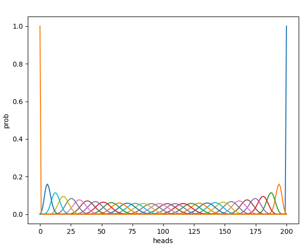
It isn't enough. See plot. Also, 200 not being enough flips is part of what makes this interesting. With a million flips, this would pretty much just be the exact case. The fact that it's only 200 flips gives you a tradeoff in how many label_bits to include.

[-]Alfred Harwood4mo40

Thanks for the clarifications, that all makes sense. I will keep thinking about this!

[-]Donald Hobson4mo40

Here is the probability density function for heads plotted for each of your coins.

python code

import numpy as np
l=np.linspace(0,1,32)
def f(a):
a=np.array([a,1-a])
b=a
for i in range(199):
b=np.convolve(b,a)
return b

q=np.arange(201)
import matplotlib.pyplot as plt
ff=[f(i) for i in l]
plt.plot(ff);plt.show()

for i in ff:
_=plt.plot(q,i)

plt.show()
plt.xlabel("heads")
Text(0.5, 0, 'heads')
plt.ylabel("prob")
Text(0, 0.5, 'prob')
for i in ff:
_=plt.plot(q,i)

plt.show()

[-]David Johnston4mo50

I've thought about it a bit, I have a line of attack for a proof, but there's too much work involved in following it through to an actual proof so I'm going to leave it here in case it helps anyone.

I'm assuming everything is discrete so I can work with regular Shannon entropy.

Consider the range of the function $g_{1} : λ \mapsto P (X_{1} | Λ = λ)$ and $R_{2}$ defined similarly. Discretize $R_{1}$ and $R_{2}$ (chop them up into little balls). Not sure which metric to use, maybe TV.

Define $Λ_{1}^{'} (λ)$ to be the index of the ball into which $P (X_{1} | Λ = λ)$ falls, $Λ_{2}^{'}$ similar. So if $d (P (X_{1} | Λ = a), P (X_{1} | Λ = b))$ is sufficiently small, then $Λ_{1}^{'} (a) = Λ_{1}^{'} (b)$ .

By the data processing inequality, conditions 2 and 3 still hold for $Λ^{'} = (Λ_{1}^{'}, Λ_{2}^{'})$ . Condition 1 should hold with some extra slack depending on the coarseness of the discretization.

It takes a few steps, but I think you might be able to argue that, with high probability, for each $X_{2} = x_{2}$ , the random variable $Q_{1} := P (X_{1} | Λ_{1}^{'})$ will be highly concentrated (n.b. I've only worked it through fully in the exact case, and I think it can be translated to the approximate case but I haven't checked). We then invoke the discretization to argue that $H (Λ_{1}^{'} | X_{1})$ is bounded. The intuition is that the discretization forces nearby probabilities to coincide, so if $Q_{1}$ is concentrated then it actually has to "collapse" most of its mass onto a few discrete values.

We can then make a similar argument switching the indices to get $H (Λ_{2}^{'} | X_{2})$ bounded. Finally, maybe applying conditions 2 and 3 we can get $H (Λ_{1}^{'} | X_{2})$ bounded as well, which then gives a bound on $H (Λ | X_{i})$ .

I did try feeding this to Gemini but it wasn't able to produce a proof.

[-]J Bostock4mo70

I've been working on the reverse direction: chopping up by clustering the points (treating each distribution as a point in distribution space) given by $P [Λ | X = x]$ , optimizing for a deterministic-in- $X$ latent $Δ = Δ (X)$ which minimizes $D_{K L} (P [Λ | X] | | P [Λ | Δ (X)])$ .

This definitely separates $X_{1}$ and $X_{2}$ to some small error, since we can just use $Δ$ to build a distribution over $Λ$ which should approximately separate $X_{1}$ and $X_{2}$ .

To show that it's deterministic in $X_{1}$ (and by symmetry $X_{2}$ ) to some small error, I was hoping to use the fact that---given $X_{1}$ --- $X_{2}$ has very little information about $Λ$ , so it's unlikely that $P [Λ | X_{1}]$ is in a different cluster to $P [Λ | X_{1}, X_{2}]$ . This means that $P [Δ | X_{1}]$ would just put most of the weight on the cluster containing $P [Λ | X_{1}]$ .

A constructive approach for $Δ$ would be marginally more useful in the long-run, but it's also probably easier to prove things about the optimal $Δ$ . It's also probably easier to prove things about $Δ$ for a given number of clusters $| Δ |$ , but then you also have to prove things about what the optimal value of $| Δ |$ is.

[-]johnswentworth4mo70

Sounds like you've correctly understood the problem and are thinking along roughly the right lines. I expect a deterministic function of won't work, though.

Hand-wavily: the problem is that, if we take the latent to be a deterministic function $Δ (X)$ , then $P [X | Δ (X)]$ has lots of zeros in it - not approximate-zeros, but true zeros. That will tend to blow up the KL-divergences in the approximation conditions.

I'd recommend looking for a function $Δ (Λ)$ . Unfortunately that does mean that low entropy of $Δ (Λ)$ given $X$ has to be proven.

[-]Alex Gibson1mo92

I'm confused by this. The KL term we are looking at in the deterministic case is
, right?

For simplicity, we imagine we have finite discrete spaces. Then this would blow up if $P [X = (x_{1}, x_{2}), Λ = λ] \neq 0$ , and $P [Λ = λ] P [X_{1} = x_{1} | Λ = λ] P [X_{2} = x_{2} | Λ = λ] = 0$ . But this is impossible, because any of the terms in the product being 0 imply that $P [X = (x_{1}, x_{2}), Λ = λ]$ is $0$ .

Intuitively, we construct an optimal code for encoding the distribution $P [Λ] P [X_{1} | Λ] P [X_{2} | Λ]$ , and the KL divergence measures how many more bits on average we need to encode a message than optimal, if the true distribution is given by $P [X, Λ]$ . Issues occur when but the true distribution $P [X, Λ]$ takes on values which never occur according to $P [Λ] P [X_{1} | Λ] P [X_{2} | Λ]$ , i.e: the optimal code doesn't account for those values potentially occurring.

Potentially there are subtleties when we have continuous spaces. In any case I'd be grateful if you're able to elaborate.

[-]johnswentworth1mo92

Yeah, I've since updated that deterministic functions are probably the right thing here after all, and I was indeed wrong in exactly the way you're pointing out.

[-]J Bostock4mo41

Huh, I had vaguely considered that but I expected any terms to be counterbalanced by $P [X, Δ (X)] = 0$ terms, which together contribute nothing to the KL-divergence. I'll check my intuitions though.

I'm honestly pretty stumped at the moment. The simplest test case I've been using is for $X_{1}$ and $X_{2}$ to be two flips of a biased coin, where the bias is known to be either $k$ or $1 - k$ with equal probability of either. As $k$ varies, we want to swap from $Δ ≅ Λ$ to the trivial case $| Δ | = 1$ and back. This (optimally) happens at around $k = 0.08$ and $k = 0.92$ . If we swap there, then the sum of errors for the three diagrams of $Δ$ does remain less than $2 (ϵ + ϵ + ϵ)$ at all times.

Likewise, if we do try to define $Δ (X)$ , we need to swap from a $Δ$ which is equal to the number of heads, to $| Δ | = 1$ , and back.

In neither case can I find a construction of $Δ (X)$ or $Δ (Λ)$ which swaps from one phase to the other at the right time! My final thought is for $Δ$ to be some mapping $Λ \to P (Λ)$ consisting of a ball in probability space of variable radius (no idea how to calculate the radius) which would take $k \to {k}$ at $k \approx 1$ and $k \to {k, 1 - k}$ at $k \approx 0.5$ . Or maybe you have to map $Λ \to P (X)$ or something like that. But for now I don't even have a construction I can try to prove things for.

Perhaps a constructive approach isn't feasible, which probably means I don't have quite the right skillset to do this.

[-]J Bostock4mo*40

OK so some further thoughts on this: suppose we instead just partition the values of directly by something like a clustering algorithm, based on $D_{K L}$ in $P [X | Λ]$ space, and take $Δ (Λ)$ just be the cluster that $λ$ is in:

Assuming we can do it with small clusters, we know that $P [X | Λ] \approx P [X | Δ]$ is pretty small, so $D_{K L} (P [X] | | P [X | Δ])$ is also small.

And if we consider $X_{2} \leftarrow X_{1} \to Λ$ , this tells us that learning $X_{1}$ restricts us to a pretty small region of $P [X_{2}]$ space (since $P [X_{2} | X_{1}] \approx P [X_{2} | X_{1}, Λ]$ ) so $Δ$ should be approximately deterministic in $X_{1}$ . This second part is more difficult to formalize, though.

Edit: The real issue is whether or not we could have lots of $Λ$ values which produce the same distribution over $X_{2}$ but different distributions over $X_{1}$ , and all be pretty likely given $X_{1} = x_{1}$ for some $x_{1}$ . I think this just can't really happen for probable values of $x_{1}$ , because if these values of $λ$ produce the same distribution over $X_{2}$ , but different distributions over $X_{1}$ , then that doesn't satisfy $X_{1} \leftarrow X_{2} \to Λ$ , and secondly because if they produced wildly different distributions over $X_{1}$ , then that means they can't all have high values of $P [X_{1} = x_{1} | Λ = λ]$ , and so they're not gonna have high values of $P [Λ = λ | X_{1} = x_{1}]$ .

[-]johnswentworth4mo*40

Here's a trick which might be helpful for anybody tackling the problem.

First, note that is always a sufficient statistic of $Λ$ for $X$ , i.e.

$Λ \to f (Λ) \to X$

Now, we typically expect that the lower-order bits of $f (Λ)$ are less relevant/useful/interesting. So, we might hope that we can do some precision cutoff on $f (Λ)$ , and end up with an approximate suficient statistic, while potentially reducing the entropy (or some other information content measure) of $f (Λ)$ a bunch. We'd broadcast the cutoff function like this:

$g (Λ) := precison_cutoff (f (Λ)) = (x \mapsto precision_cutoff (P [X = x | Λ]))$

Now we'll show a trick for deriving $D_{K L}$ bounds involving $g (Λ)$ .

First note that

$E [D_{K L} (P [X | Λ] | | P [X | g (Λ)])] \leq E [D_{K L} (P [X | Λ] | | g (Λ))]$

This is a tricky expression, so let's talk it through. On the left, $g (Λ)$ is treated informationally; it's just a generic random variable constructed as a generic function of $Λ$ , and we condition on that random variable in the usual way. On the right, the output-value of $g$ is being used as a distribution over $X$ .

The reason this inequality holds is because a Bayes update is the "best" update one can make, as measured by expected $D_{K L}$ . Specifically, if I'm given the value of any function $g (Λ)$ , then the distribution $Q$ (as a function of $g (Λ))$ which minimizes $E [D_{K L} (P [X | Λ] | | Q)]$ is $P [X | g (Λ)]$ . Since $P [X | g (Λ)]$ minimizes that expected $D_{K L}$ , any other distribution over $X$ (as a function of $g (Λ)$ ) can only do "worse" - including $g (Λ)$ itself, since that's a distribution over $X$ , and is a function of $g (Λ)$ .

Plugging in the definition of $g$ , that establishes

$E [D_{K L} (P [X | Λ] | | P [X | g (Λ)])] \leq E [D_{K L} (P [X | Λ] | | (x \mapsto precision_cutoff (P [X = x | Λ])))]$

Then the final step is to use the properties of whatever $precision_cutoff$ function one chose, to establish that $E [D_{K L} (P [X | Λ] | | (x \mapsto precision_cutoff (P [X = x | Λ])))]$ can't be too far from $E [D_{K L} (P [X | Λ] | | P [X | Λ])]$ , i.e. 0. That produces an upper bound on $E [D_{K L} (P [X | Λ] | | P [X | g (Λ)])]$ , where the bound is 0 + (whatever terms came from the precision cutoff).

[-]johnswentworth4mo20

@Alfred Harwood @David Johnston

If anyone else would like to be tagged in comments like this one on this post, please eyeball-react on this comment. Alfred and David, if you would like to not be tagged in the future, please say so.

[-]Arjun Pitchanathan3mo*30

Epistemic status: Quick dump of something that might be useful to someone. o3 and Opus 4 independently agree on the numerical calculations for the bolded result below, but I didn't check the calculations myself in any detail.

When we say "roughly", e.g. or $3 ϵ$ would be fine; it may be a judgement call on our part if the bound is much larger than that.

Let $Y \sim Ber (p)$ . With probability $r$ , set $Z := X$ , and otherwise draw $Z \sim Ber (p)$ . Let $Y \sim Ber (1 / 2)$ . Let $A = X \oplus Y$ and $B = Y \oplus Z$ . We will investigate latents for $(A, B)$ .

Set $Λ := Y$ , then note that the stochastic error $ϵ := I (A; Y | B)$ ) because $Y$ induces perfect conditional independence and symmetry of $A$ and $B$ . Now compute the deterministic errors of $Λ := Y$ , $Λ := 0$ , $Λ := A$ , which are equal to $H (Y ∣ A), I (A; B), H (A | B)$ respectively.

Then it turns out that with $p := 0.9, r := 0.44$ , all of these latents have error greater than $5 ϵ$ , if you believe this claude opus 4 artifact (full chat here, corroboration by o3 here). Conditional on there not being some other kind of latent that gets better deterministic error, and the calculations being correct, I would expect that a bit more fiddling around could produce much better bounds, say $10 ϵ$ or more, since I think I've explored very little of the search space.

e.g. one could create more As and Bs by either adding more Ys, or more Xs and Zs. Or one could pick the probabilities $p, r$ out of some discrete set of possibilities instead of having them be fixed.

[-]johnswentworth2mo53

Set , then note that the stochastic error $ϵ := I (A; Y | B)$ ) because $Y$ induces perfect conditional independence and symmetry of $A$ and $B$ .

I don't think Y induces perfect conditional independence? Conditional on Y, we have:

(Probability r) A = B, else
(Probability 1 - r) A and B are independent

... which means that learning the value of A tells me something about the value of B, conditional on Y (specifically, B is more likely to have the same value A had).

Am I missing something here?

(Also, for purposes of me tracking how useful LLMs are for research: assuming I'm not missing something and this was a mistake, was the mistake originally made by you or an LLM?)

[-]Arjun Pitchanathan1mo40

Yeah, my comment went through a few different versions and that statement doesn't apply to the final setting. I should've checked it better before hitting submit, sorry. I only used LLMs for writing code for numerical calculations, so the error is mine. ^[1]

I think that I didn't actually use this claim in the numerical calculations, so I'd hope that the rest of the comment continues to hold. I had hoped to verify that before replying, but given that it's been two weeks already, I don't know when I'll manage to get to it.

^{^}
I did try to see if it could write a message explaining the claim, but didn't use that

[-]Arjun Pitchanathan1mo*30

To check my understanding: for random variables , the stochastic error of a latent $Λ$ is the maximum among $I (A; B | Λ), I (A; Λ | B), I (B; Λ | A)$ . The deterministic error is the maximum among $I (A; B ∣ Λ), H (Λ | A), H (Λ | B)$ . If so, the claim in my original comment holds -- I also wrote code (manually) to verify. Here's the fixed claim:

Let $X \sim Ber (p)$ . With probability $r$ , set $Z := X$ , and otherwise draw $Z \sim Ber (p)$ . Let $Y \sim Ber (1 / 2)$ . Let $A = X \oplus Y$ and $B = Y \oplus Z$ . We will investigate latents for $(A, B)$ . Let $ϵ$ be the stochastic error of latent $Λ := Y$ . Now compute the deterministic errors of each of the latents $X$ , $Y$ , $Z$ , $A$ , $B$ , $A \oplus B$ , $X \oplus Y \oplus Z$ . Then for $p := 0.9, r := 0.44$ , all of these latents have deterministic error greater than $5 ϵ$ .

It should be easy to modify the code to consider other latents. I haven't thought much about proving that there aren't any other latents better than these, though.

[-]Arjun Pitchanathan1mo*30

On this particular example you can achieve deterministic error with latent $A \land B$ , but it seems easy to find other examples with ratio > 5 (including over latents $A \land B, A \lor B$ ) in the space of distributions over $(X, Y, Z)$ with a random-restart hill-climb. Anyway, my takeaway is that if you think you can derandomize latents in general you should probably try to derandomize the latent $Λ := Y$ for variables $A := X \oplus Y$ , $B := Z \oplus Y$ for distributions over boolean variables $X, Y, Z$ .

(edited to fix typo in definition of $B$ )

[-]Arjun Pitchanathan1mo*30

My impression is that prior discussion focused on discretizing . $Λ$ is already boolean here, so if the hypothesis is true then it's for a different reason.

[-]David Johnston4mo*10

Your natural latents seem to be quite related to the common construction IID variables conditional on a latent - in fact, all of your examples are IID variables (or "bundles" of IID variables) conditional on that latent. Can you give me an interesting example of a natural latent that is not basically the conditionally IID case?

(I was wondering if the extensive literature on the correspondence between De Finetti type symmetries and conditional IID representations is of any help to your problem. I'm not entirely sure if it is, given that mostly addresses the issue of getting from a symmetry to a conditional independence, whereas you want to get from one conditional independence to another, but it's plausible some of the methods are applicable)

[-]johnswentworth4mo20

A natural latent is, by definition, a latent which satisfies two properties. The first is that the observables are IID conditional on the latent, i.e. the common construction you're talking about. That property by itself doesn't buy us much of interest, for our purposes, but in combination with the other property required for a natural latent, it buys quite a lot.