Natural latents are a relatively elegant piece of math which we figured out over the past year, in our efforts to boil down and generalize various results and examples involving natural abstraction. In particular, this new framework handles approximation well, which was a major piece missing previously. This post will present the math of natural latents, with a handful of examples but otherwise minimal commentary. If you want the conceptual story, and a conceptual explanation for how this might connect to various problems, that will probably be in a future post.

While this post is not generally written to be a "concepts" post, it is generally written in the hope that people who want to use this math will see how to do so.

2-Variable Theorems

This section will present a simplified but less general version of all the main theorems of this post, in order to emphasize the key ideas and steps.

Simplified Fundamental Theorem

Suppose we have:

• A distribution $P\left[X\right]$ over random variables $X=(X_1,X_2)$
• A latent variable $\Lambda$ which induces independence between $X_1$ and $X_2$ (first diagram below)
• Another latent variable ${\Lambda }^{\prime }$ about which $X_1$ and $X_2$ give the same information (second diagram below)

Further, assume that $X$ mediates between $\Lambda$ and ${\Lambda }^{\prime }$ (third diagram below). This last assumption can typically be satisfied by construction in the minimality/maximality theorems below.

Then, claim: $\Lambda$ mediates between ${\Lambda }^{\prime }$ and $X$.

Intuition

Picture $\Lambda$ as a pipe between $X_1$ and $X_2$. The only way any information can get from $X_1$ to $X_2$ is via that pipe (that’s the first diagram). ${\Lambda }^{\prime }$ is a piece of information which is present in both $X_1$ and $X_2$ - something we can learn from either of them (that’s the second pair of diagrams). Intuitively, the only way that can happen is if the information ${\Lambda }^{\prime }$ went through the pipe - meaning that we can also learn it from $\Lambda$.

The third diagram rules out three-variable interactions which could mess up that intuitive picture - for instance, the case where one bit of ${\Lambda }^{\prime }$ is an xor of some independent random bit of $\Lambda$ and a bit of $X$.

Qualitative Example

Let $X_1$ and $X_2$ be the low-level states of two spatially-separated macroscopic chunks of an ideal gas at equilibrium. By looking at either of the two chunks, I can tell whether the temperature is above 50°C; call that ${\Lambda }^{\prime }.$ More generally, the two chunks are independent given the pressure and temperature of the gas; call that $\Lambda$.

Notice that ${\Lambda }^{\prime }$ is a function of $\Lambda$, i.e. I can compute whether the temperature is above 50°C from the pressure and temperature itself, so $\Lambda$ mediates between ${\Lambda }^{\prime }$ and $X$.

Some extensions of this example:

• We could add more information to $\Lambda$. For instance, $\Lambda$ could be the pressure and temperature and also the outcome of a die roll unrelated to the gas. Or, $\Lambda$ could be the entire low-level state of one of the two chunks.
• We could remove information from ${\Lambda }^{\prime }.$ For instance, ${\Lambda }^{\prime }$ could be a bit indicating whether the temperature is above 100°C

Intuitive mental picture: in general, $\Lambda$ can’t have “too little” information; it needs to include all information shared (even partially) across $X_1$ and $X_2$. ${\Lambda }^{\prime },$ on the other hand, can’t have “too much” information; it can only include information which is fully shared across $X_1$ and $X_2$.

Proof

This is a diagrammatic proof; see Some Rules For An Algebra Of Bayes Nets for how to read it. (That post also walks through a version of this same proof as an example, so you should also look there if you want a more detailed walkthrough.)

(Throughout this post, $X_{\overline{i}}$ denotes all components of $X$ except for $X_i$.) 

Approximation

If the starting diagrams are satisfied approximately (i.e. they have small KL-divergence from the underlying distribution), then the final diagram is also approximately satisfied (i.e. has small KL-divergence from the underlying distribution). We can find quantitative bounds by propagating error through the proof: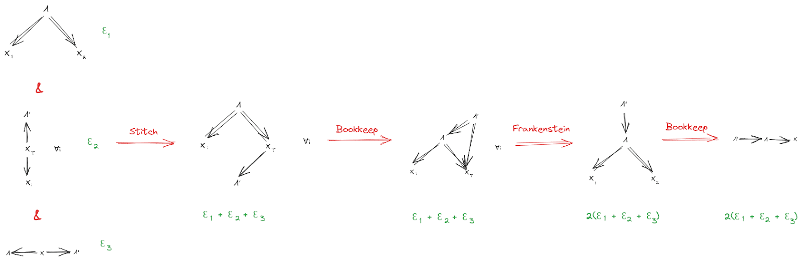

Again, see the Algebra of Bayes Nets post for an unpacking of this notation and the proofs for each individual step.

Qualitative Example

Note that our previous example realistically involved approximation: two chunks of an ideal gas won’t be exactly independent given pressure and temperature. But they’ll be independent to a very (very) tight approximation, so our conclusion will also hold to a very tight approximation.

Quantitative Example

Suppose I have a biased coin, with bias $\theta$. Alice flips the coin 1000 times, then takes the median of her flips. Bob also flips the coin 1000 times, then takes the median of his flips. We’ll need a prior on $\theta$, so for simplicity let’s say it’s uniform on [0, 1].

Intuitively, so long as bias $\theta$ is unlikely to be very close to ½, Alice and Bob will find the same median with very high probability. So:

• Let $X_1$ be Alice’ 1000 flips, and $X_2$ be Bob’s 1000 flips.
• Let $\Lambda$ be the bias $\theta$. Note that the flips are independent given $\theta$, satisfying our first condition exactly.
• Let ${\Lambda }^{\prime }$ be the median computed by either Bob or Alice (we’re assuming they are the same with high probability). Since the same median can be computed with high probability from either $X_1$ or $X_2$, our second condition is approximately satisfied.
• Since the median is computed as a deterministic function of $X$, our third condition is satisfied exactly.

The fundamental theorem will then say that the bias approximately mediates between the median (either Alice’ or Bob’s) and the coinflips $X$.

To quantify the approximation on the fundamental theorem, we first need to quantify the approximation on the second condition (the other two conditions hold exactly in this example, so their $ϵ$'s are 0). Let’s take ${\Lambda }^{\prime }$ to be Alice’ median. Alice’ flips mediate between Bob’s flips and the median exactly (i.e. $X_2\to X_1\to {\Lambda }^{\prime }$), but Bob’s flips mediate between Alice’ flips and the median (i.e. $X_1\to X_2\to {\Lambda }^{\prime }$) only approximately. Let’s compute that $D_{KL}$:

$D_{KL}\left(P\right[X_1,X_2,{\Lambda }^{\prime }\left]||P\right[X_1\left]P\right[X_2|X_1\left]P\right[{\Lambda }^{\prime }|X_2\left]\right)$

$=-{\sum }_{X_1,X_2}P[X_1,X_2]lnP\left[{\Lambda }^{\prime }\right(X_1\left)|X_2\right]$

$=E\left[H\right({\Lambda }^{\prime }\left(X_1\right)|X_2\left)\right]$

This is a dirichlet-multinomial distribution, so it will be cleaner if we rewrite in terms of $N_1:=\sum X_1$, $N_2:=\sum X_2$, and $n:=1000$. ${\Lambda }^{\prime }$ is a function of $N_1$, so the $D_{KL}$ is

$=E\left[H\right({\Lambda }^{\prime }\left(N_1\right)|N_2\left)\right]$

Assuming I simplified the gamma functions correctly, we then get:

$P\left[N_2\right]=\frac{1}{n+1}$ (i.e. uniform over 0, …, n)

$P\left[N_1|N_2\right]=\frac{\Gamma (n+2)}{\Gamma (N_2+1)\Gamma (n-N_2+1)}\frac{\Gamma (n+1)}{\Gamma (N_1+1)\Gamma (n-N_1+1)}\frac{\Gamma (N_1+N_2+1)\Gamma (2n-N_1-N_2+1)}{\Gamma (2n+2)}$

$P\left[{\Lambda }^{\prime }\right(N_1)=0|N_2]={\sum }_{n_1<500}P\left[N_1|N_2\right]$

$P\left[{\Lambda }^{\prime }\right(N_1)=1|N_2]={\sum }_{n_1>500}P\left[N_1|N_2\right]$

… and there’s only ${1001}^2$ values of $(N_1,N_2)$, so we can combine those expressions with a python script to evaluate everything:

import numpy as np
from scipy.special import gammaln, logsumexp, xlogy

n = 1000
p_N2 = np.ones(n+1)/(n+1)
N1 = np.outer(np.arange(n + 1), np.ones(n + 1))
N2 = np.outer(np.ones(n + 1), np.arange(n + 1))
# logP[N1|N2]; we're tracking log probs for numerical stability
lp_N1_N2 = (gammaln(n + 2) - gammaln(N2 + 1) - gammaln(n - N2 + 1) +
            gammaln(n + 1) - gammaln(N1 + 1) - gammaln(n - N1 + 1) +
            gammaln(N1 + N2 + 1) + gammaln(2*n - N1 - N2 + 1) - gammaln(2*n + 2))

# logP[\Lambda' = 0|N2] and logP[\Lambda' = 1|N2]
lp_lam0_N2 = logsumexp(lp_N1_N2[:500], axis=0)
lp_lam1_N2 = logsumexp(lp_N1_N2[500:], axis=0)

p_lam0_N2 = np.exp(lp_lam0_N2)
p_lam1_N2 = np.exp(lp_lam1_N2)

print(p_lam0_N2 + p_lam1_N2)  # Check: these should all be 1.0

# ... aaaand then it's just the ol' -p * logp to get the expected entropy E[H(\Lambda')|N2]
H = - np.sum(p_lam0_N2 * lp_lam0_N2 * p_N2) - np.sum(p_lam1_N2 * lp_lam1_N2 * p_N2)
print(H / np.log(2))  # Convert to bits

The script spits out H = 0.058 bits. Sanity check: the main contribution to the entropy should be when $\theta$ is near 0.5, in which case the median should have roughly 1 bit of entropy. How close to 0.5? Well, with $n$ data points, posterior uncertainty should be of order $\frac{1}{\sqrt{n}}$, so the estimate of $\theta$ should be precise to roughly $\frac{1}{30}\approx .03$ in either direction. $\theta$ is initially uniform on [0, 1], so distance 0.03 in either direction around 0.5 covers about 0.06 in prior probability, and the entropy should be roughly that times 1 bit, so roughly 0.06 bits. Which is exactly what we found (closer than this sanity check had any business being, really); sanity check passes.

Returning to the fundamental theorem: ${ϵ}_1$ is 0, ${ϵ}_3$ is 0, ${ϵ}_2$ is roughly 0.058 bits. So, the theorem says that the coin’s true bias approximately mediates between the coinflips and Alice’ median, to within $2({ϵ}_1+{ϵ}_2+{ϵ}_3)\approx$ 0.12 bits. 

Exercise: if we track the $ϵ$’s a little more carefully through the proof, we’ll find that we can actually do somewhat better in this case. Show that, for this example, the coin’s true bias approximately mediates between the coinflips and Alice’ median to within ${ϵ}_2$, i.e. roughly 0.058 bits.

Extension: More Stuff In The World

Let’s add another random variable $Z$ to the setup, representing other stuff in the world. $Z$ can have any relationship at all with $X$, but $\Lambda$ must still induce independence between $X_1$ and $X_2$. Further, $Z$ must not give any more information about ${\Lambda }^{\prime }$ than was already available from $X_1$ or $X_2$. Diagrams:

Then, as before, we conclude

For instance, in our ideal gas example, we could take $Z$ to be the rest of the ideal gas (besides the two chunks $X_1$ and $X_2$). Then, our earlier conclusions still hold, even though there’s “more stuff” physically in between $X_1$ and $X_2$ and interacting with both of them.

The proof goes through much like before, with an extra Z dangling everywhere:

And, as before, we can propagate error through the proof to obtain an approximate version:

Natural Latents

Suppose that a single latent variable $\Lambda$ (approximately) satisfies both the first two conditions of the Fundamental Theorem, i.e.

We call these the “naturality conditions”. If $\Lambda$ (approximately) satisfies both conditions, then we call $\Lambda$ a “natural latent”.

Example: if $X_1$ and $X_2$ are two spatially-separated mesoscopic chunks of an ideal gas, then the tuple (pressure, temperature) is a natural latent between the two. The first property (“mediation”) applies because pressure and temperature together determine all the intensive quantities of the gas (like e.g. density), and the low-level state of the gas is (approximately) independent across spatially-separated chunks given those quantities. The second property (“insensitivity”) applies because the pressure and temperature can be precisely and accurately estimated from either chunk.

The Resample

Recall earlier that we said the condition

would be satisfied by construction in our typical use-case. It’s time for that construction.

The trick: if we have a natural latent $\Lambda$, then construct a new natural latent by resampling $\Lambda$ conditional on $X$ (i.e. sample from $P\left[\Lambda |X\right]$), independently of whatever other stuff ${\Lambda }^{\prime }$ we’re interested in. The resampled $\Lambda$ will have the same joint distribution with $X$ as $\Lambda$ does, so it will also be a natural latent, but it won’t have any “side-channel” interactions with other variables in the system - all of its interactions with everything else are mediated by $X$, by construction.

From here on out, we’ll usually assume that natural latents have been resampled (and we’ll try to indicate that with the phrase “resampled natural latent”).

Minimality & Maximality

Finally, we’re ready for our main theorems of interest about natural latents.

Assume that $\Lambda$ is a resampled natural latent over $X$. Take any other latent ${\Lambda }^{\prime }$ about which $X_1$ and $X_2$ give (approximately) the same information, i.e.

Then, by the fundamental theorem:

So $\Lambda$ is, in this sense, the “most informative” latent about which $X_1$ and $X_2$ give the same information:

$X_1$ and $X_2$ give (approximately) the same information about $\Lambda$, and for any other latent ${\Lambda }^{\prime }$ such that $X_1$ and $X_2$ give (approximately) the same information about ${\Lambda }^{\prime },$ $\Lambda$ tells us (approximately) everything which ${\Lambda }^{\prime }$ does about $X$ (and possibly more). This is the “maximality condition”.

Flipping things around: take any other latent ${\Lambda }^{\prime \prime }$ which (approximately) induces independence between $X_1$ and $X_2$:

By the fundamental theorem:

So $\Lambda$ is, in this sense, the “least informative” latent which induces independence between $X_1$ and $X_2$:

$\Lambda$ (approximately) induces independence between $X_1$ and $X_2$, and for any other latent ${\Lambda }^{\prime \prime }$ which (approximately) induces independence between $X_1$ and $X_2$, ${\Lambda }^{\prime \prime }$ tells us (approximately) everything which $\Lambda$ does about $X$ (and possibly more). This is the “minimality condition”.

Further notes:

• The minimality condition implies the natural latent conditions. Proof: take ${\Lambda }^{\prime \prime }$ to be either $X_1$ or $X_2$.
• Both minimality and maximality imply a unique standard form (see appendix), so any resampled natural latent in standard form is also the unique natural and minimal and maximal latent in standard form. (In the approximate case, this becomes approximate uniqueness.) Furthermore, any natural latent can be transformed into standard form (as the phrase “standard form” implies).
• In standard form, a natural latent is always approximately a deterministic function of $X$. Specifically: $\Lambda \left(X\right)\approx {\prod }_i(x^{\prime }\mapsto P[X_i=x_i^{\prime }|X_{\overline{i}}\left]\right)$.
• Natural and minimal latents do not always exist, and maximal latents sometimes exist in cases where natural/minimal latents don’t. (For example, if $X_1$ and $X_2$ are two flips of a biased coin of unknown bias, then no natural latent exists to a good approximation. Intuitively, it's because we don't have enough data to precisely identify the bias which mediates between the datapoints.)
• Basically everything about approximation and other parts of the world carries over to naturality/minimality/maximality.

Example

In the ideal gas example, two chunks of gas are independent given (pressure, temperature), and (pressure, temperature) can be precisely estimated from either chunk. So, (pressure, temperature) is (approximately) a natural latent across the two chunks of gas. The resampled natural latent would be the (pressure, temperature) estimated by looking only at the two chunks of gas.

If there is some other latent which induces independence between the two chunks (like, say, the low-level state trajectory of all the gas in between the two chunks), then the (pressure, temperature) estimated from the two chunks of gas must (approximately) be a function of that latent. And, if there is some other latent about which the two chunks give the same information (like, say, a bit which is 1 if-and-only-if temperature is above 50 °C), then (pressure, temperature) estimated from the two chunks of gas must (approximately) also give that same information.

General Case

Now we move on to more-than-two variables. The proofs generally follow the same structure as the two-variable case, just with more bells and whistles, and are mildly harder to intuit. This time, rather than ease into it, we’ll include approximation and other parts of the world ($Z$) in the theorems upfront.

The Fundamental Theorem

Suppose we have:

• A distribution $P[X,Z]$ over random variables $X_1$, …, $X_n$, $Z$
• A latent variable $\Lambda$ which induces independence between all $X_i$ (first diagram below)
• A latent variable ${\Lambda }^{\prime }$ which is insensitive to any $X_i$ given all the others (second diagram below)

Further, assume that $(X,Z)$ mediates between $\Lambda$ and ${\Lambda }^{\prime }$ (third diagram below). This last assumption will be exactly satisfied by construction in the minimality/maximality theorems below.

Then, claim: $\Lambda$ mediates between ${\Lambda }^{\prime }$ and $(X,Z)$.

The diagrammatic proof, with approximation:

Note that the error bound is somewhat unimpressive, since it scales with the system size. We can strengthen the approximation mainly by using a stronger insensitivity condition for ${\Lambda }^{\prime }$ - for instance, if ${\Lambda }^{\prime }$ is insensitive to either of two halves of the system, then we can reuse the error bounds from the simplified 2-variable case earlier.

Natural Latents

Suppose a single latent $\Lambda$ (approximately) satisfies both the main conditions

We call these the “naturality conditions”, and we call $\Lambda$ a (approximate) “natural latent” over $X$.

The resample step works exactly as before: we’ll generally assume that $\Lambda$ has been resampled conditional on $X$, and try to indicate that with the phrase “resampled natural latent”.

Minimality & Maximality

Assume $\Lambda$ is a resampled natural latent over $X$. Take any other latent ${\Lambda }^{\prime }$ about which $X_{\overline{i}}$ gives (approximately) the same information as $(X,Z)$ for any $i$:

By the fundamental theorem:

So $\Lambda$ is, in this sense, the “most informative” latent about which all $X_{\overline{i}}$ give the same information:

All $X_{\overline{i}}$ give (approximately) the same information about $\Lambda$, and for any other latent ${\Lambda }^{\prime }$ such that all $X_{\overline{i}}$ give (approximately) the same information about ${\Lambda }^{\prime },$ $\Lambda$ tells us (approximately) everything which ${\Lambda }^{\prime }$ does about $X$ (and possibly more). This is the “maximality condition”.

Flipping things around: take any other latent ${\Lambda }^{\prime \prime }$ which (approximately) induces independence between components of $X$. By the fundamental theorem:

So $\Lambda$ is, in this sense, the “least informative” latent which induces independence between components of $X$:

$\Lambda$ (approximately) induces independence between components of $X$, and for any other latent ${\Lambda }^{\prime \prime }$ which (approximately) induces independence between components of $X$, ${\Lambda }^{\prime \prime }$ tells us (approximately) everything which $\Lambda$ does about $X$ (and possibly more). This is the “minimality condition”.

Much like the simplified 2-variable case:

• The minimality condition implies the natural latent conditions. Proof: take ${\Lambda }^{\prime \prime }$ to be $X_{\overline{i}}$, for each $i$.
• Both minimality and maximality imply an approximately unique standard form (see appendix), so any natural latent in standard form is also the approximately unique natural and minimal and maximal latent in standard form. Furthermore, any natural latent can be transformed into standard form (as the phrase “standard form” implies).
• In standard form, a natural latent is always approximately a deterministic function of $X$. Specifically: $\Lambda \left(X\right)\approx {\prod }_i(x^{\prime }\mapsto P[X_i=x_i^{\prime }|X_{\overline{i}}\left]\right)$.
• Natural and minimal latents do not always exist, and maximal latents sometimes exist in cases where natural/minimal latents don’t.
• Everything about approximation and other parts of the world carries over to naturality/minimality/maximality.

Example

Suppose we have a die of unknown bias, which is rolled many times - enough to obtain a precise estimate of the bias many times over. Then, the die-rolls are independent given the bias, and we can get approximately-the-same estimate of the bias while ignoring any one die roll. So, the die’s bias is an approximate natural latent. The resampled natural latent is the bias sampled from a posterior distribution of the bias given the die rolls.

One interesting thing to note in this example: imagine that, instead of resampling the bias given the die rolls, we use the average frequencies from the die rolls. Would that be a natural latent? Answer in spoiler text:

The most subtle challenges and mistakes in using natural latents tend to hinge on this point.

Other Threads

We’ve now covered the main theorems of interest. This section offers a couple of conjectures, with minimal commentary.

Universal Natural Latent Conjecture

Suppose there exists an approximate natural latent over $X_1,\dots ,X_n$. Construct a new random variable $X^{\prime },$ sampled from the distribution $(x^{\prime }\mapsto P[X_i=x_i^{\prime }|X_{\overline{i}}\left]\right)$. (In other words: simultaneously resample each $X_i$ given all the others.) Conjecture: $X^{\prime }$ is an approximate natural latent (though the approximation may not be the best possible). And if so, a key question is: how good is the approximation?

Further conjecture: a natural latent exists over $X$ if-and-only-if $X$ is a natural latent over $X^{\prime }$.(Note that we can always construct $X^{\prime }$, regardless of whether a natural latent exists, and $X$ will always exactly satisfy the first natural latent condition over $X^{\prime }$ by construction.) Again, assuming the conjecture holds at all, a key question is to find the relevant approximation bounds.

Maxent Conjecture

Assuming the universal natural latent conjecture holds, whenever there exists a natural latent $X^{\prime }$ and $X$ would approximately satisfy both of these two diagrams:

If we forget about all the context and just look at these two diagrams, one natural move is:

• Convert to undirected graphical models (in this case, just remove the arrowheads)
• Apply the Hammersley-Clifford method

… and the result would be that $P[X,X^{\prime }]$ must be of the maxent form

$\frac{1}{Z}{e}^{{\sum }_{ij}{\varphi }_{ij}(X_i,X_j^{\prime })}$

for some $\varphi$.

Unfortunately, Hammersley-Clifford requires $P[X,X^{\prime }]>0$ everywhere. Probabilities of zero are extremely load-bearing for natural latents in the exact case, and probabilities near zero are load-bearing in the approximate case; if the distribution is zero nowhere, then it can only have a natural latent if the $X_i$’s are all independent (in which case the trivial variable is a natural latent).

On the other hand, maxent sure does seem to be a theme of natural latents in e.g. physics. So the question is: does some version of this argument work? If there are loopholes, are there relatively few qualitative categories of loopholes which could be classified?

Appendix: Machinery For Latent Variables

If you get confused about things like “what exactly is a latent variable?”, this is the appendix for you.

For our purposes, a latent variable $\Lambda$ over a random variable $X$ is defined by a distribution function $(\lambda ,x\mapsto P[\Lambda =\lambda |X=x\left]\right)$ - i.e. a distribution which tells us how to sample $\Lambda$ from $X$. For instance, in the ideal gas example, the latent “average temperature” ($\Lambda$) can be defined by the distribution of average energy as a function of the gas state ($X$) - in this case a deterministic distribution, since average energy is a deterministic function of the gas state. As another example, consider the unknown bias of a die ($\Lambda$) and a bunch of rolls of the die ($X$). We would take the latent bias to be defined by the function mapping the rolls $X$ to the posterior distribution of the bias given the rolls $(\lambda \mapsto P[\Lambda =\lambda |X\left]\right)$.

So, if we talk about e.g. “existence of a latent ${\Lambda }^{\ast }$ with the following properties …”, we’re really talking about the existence of a conditional distribution function $({\lambda }^{\ast },x\mapsto P[{\Lambda }^{\ast }={\lambda }^{\ast }|X=x\left]\right)$, such that the random variable ${\Lambda }^{\ast }$ which it introduces satisfies the relevant properties. When we talk about “any latent satisfying the following properties …”, we’re really talking about any conditional distribution function $(\lambda ,x\mapsto P[\Lambda =\lambda |X=x\left]\right)$ such that the variable $\Lambda$ satisfies the relevant properties.

Toy mental model behind this way of treating latent variables: there are some variables $X$ out in the world, and those variables have some “true frequencies” $P\left[X\right]$. Different agents learn to model those true frequencies using different generative models, and those different generative models each contain their own latents. So the underlying distribution $P\left[X\right]$ is fixed, but different agents introduce different latents with different $P\left[\Lambda |X\right]$; $P\left[\Lambda |X\right]$ is taken to be definitional because it tells us everything about the joint distribution of $\Lambda$ and $X$ which is not already pinned down by $P\left[X\right]$. (This is probably not the most general/powerful mental model to use for this math, but it’s a convenient starting point.)

Standard Form of a Latent Variable

Suppose that $X$ consists of a bunch of rolls of a biased die, and a latent $\Lambda$ consists of the bias of the die along with the flip of one coin which is completely independent of the rest of the system. A different latent for the same system consists of just the bias of the die. We’d like some way to say that these two latents contain the same information for purposes of $X$.

To do that, we’ll introduce a “standard form” ${\Lambda }^{\ast }$ (relative to $X$) for any latent variable $\Lambda$:

${\Lambda }^{\ast }=(x\mapsto P[X=x|\Lambda \left]\right)$

We’ll say that a latent is “in standard form” if, when we use the above function to put it into standard form, we end up with a random variable equal to the original. So, a latent ${\Lambda }^{\ast }$ in standard form satisfies

${\Lambda }^{\ast }=(x\mapsto P[X=x|{\Lambda }^{\ast }\left]\right)$

As the phrase “standard form” suggests, putting a standard form latent into standard form leaves it unchanged, i.e. ${\Lambda }^{\ast }:=(x\mapsto P[X=x|\Lambda \left]\right)$ will satisfy ${\Lambda }^{\ast }=(x\mapsto P[X=x|{\Lambda }^{\ast }\left]\right)$ for any latent $\Lambda$; that’s a lemma of the minimal map theorem.

Conceptually: the standard form throws out all information which is completely independent of $X$, and keeps everything else. In standard statistics jargon: the likelihood function is always a minimal sufficient statistic. (See the minimal map theorem for more explanation.)