I've noticed that L0's above 100 (for the Pythia-70M model) is too high, resulting in mostly polysemantic features (though some single-token features were still monosemantic)
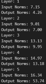
Agreed w/ Arthur on the norms of features being the cause of the higher MSE. Here are the L2 norms I got. Input is for residual stream, output is for MLP_out.
I agree that the L0's for 0_8192 are too high in later layers, though I'll note that I think this is mainly due to the cluster of high-frequency features (see the spike in the histogram). Features outside of this spike look pretty decent, and without the spike our L0s would be much more reasonable.
Here are four random features from layer 3, at a range of frequencies outside of the spike.
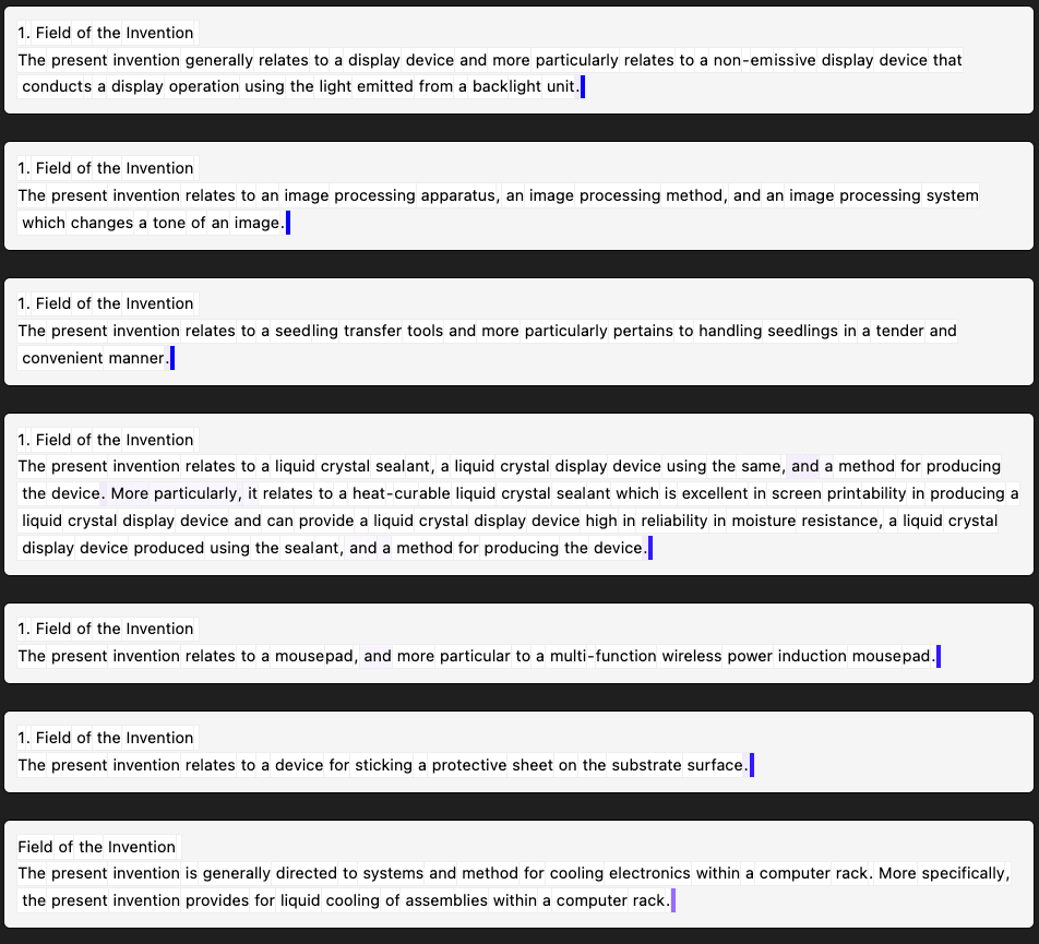
Layer 3, 0_8192, feature 138 (frequency = 0.003) activates on the newline at the end of the "field of the invention" section in patent applications. I think it's very likely predicting that the next few tokens will be "2. Description of the Related Art" (which always comes next in patents).
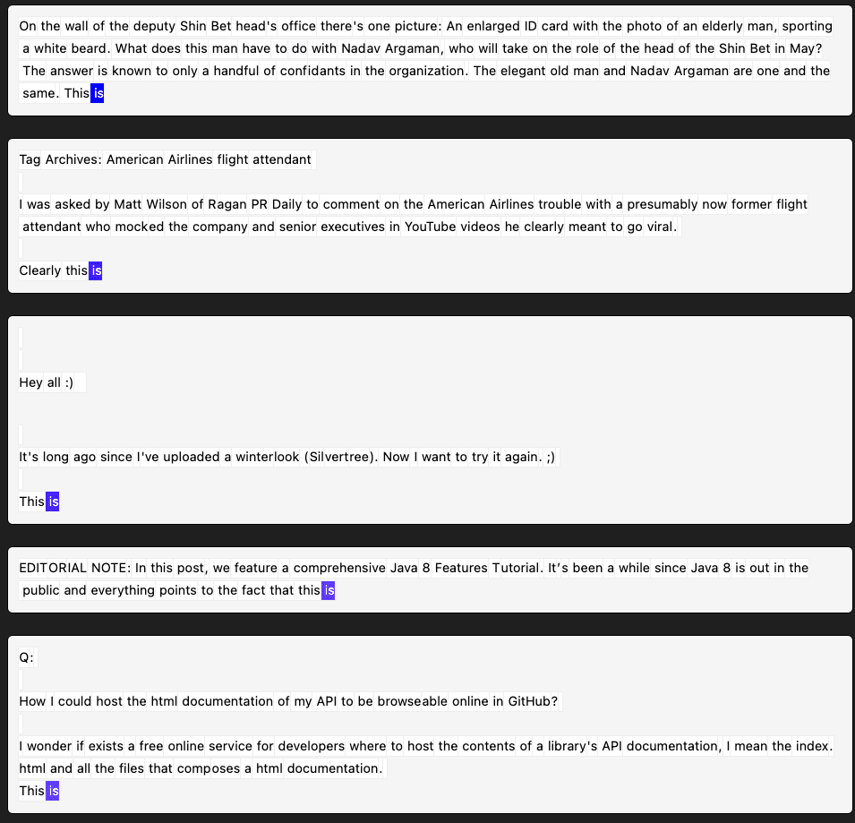
Layer 3, 0_8192, feature 27 (frequency = 0.009) seems to activate on the "is" in the phrase "this is"
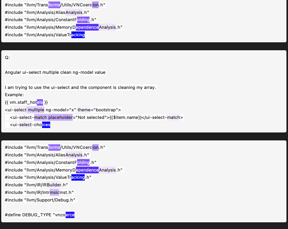
Layer 3, 0_8192, feature 4 (frequency = 0.026) looks messy at first, but on closer inspection seems to activate on the final token of multi-token words in informative file/variable names.
Layer 3, 0_8192, feature 56 (frequency = 0.035) looks very polysemantic: it's activating on certain terms in LaTeX expressions, words in between periods in urls and code, and some other random-looking stuff.
If you removed the high-frequency features to achieve some L0 norm, X, how much does loss recovered change?
If you increased the l1 penalty to achieve L0 norm X, how does the loss recovered change as well?
Ideally, we can interpret the parts of the model that are doing things, which I'm grounding out as loss recovered in this case.
Here's an experiment I'm about to do:
- Remove high-frequency features from 0_8192 layer 3 until it has L0 < 40 (the same L0 as the 1_32768 layer 3 dictionary)
- Recompute statistics for this modified dictionary.
I predict the resulting dictionary will be "like 1_32768 but a bit worse." Concretely, I'm guessing that means % loss recovered around 72%.
Results:
I killed all features of frequency larger than 0.038. This was 2041 features, and resulted in a L0 just below 40. The stats:
MSE Loss: 0.27 (worse than 1_32768)
Percent loss recovered: 77.9% (a little bit better than 1_32768)
I was a bit surprised by this -- it suggests the high-frequency features are disproportionately likely to be useful for reconstructing activations in ways that don't actually mater to the model's computation. (Though then again, maybe this is what we expect for uninterpretable features.)
It also suggests that we might be better off training dictionaries with a too-low L1 penalty and then just pruning away high-frequency features (sort of the dual operation of "train with a high L1 penalty and resample low-frequency features"). I'd be interested for someone to explore if there's a version of this that helps.
Do you apply LR warmup immediately after doing resampling (i.e. immediately reducing the LR, and then slowly increasing it back to the normal value)? In my GELU-1L blog post I found this pretty helpful (in addition to doing LR warmup at the start of training)
At the time that I made this post, no, but this has been implemented in dictionary_learning since I saw your suggestion to do so in your linked post.
As more people begin work on interpretability projects which incorporate dictionary learning, it will be valuable to have high-quality dictionaries publicly available.[1] To get the ball rolling on this, my collaborator (Aaron Mueller) and I are:
Let's discuss the dictionaries first, and then the repo.
The dictionaries
[EDIT 02/07/2024: Better dictionaries are now available at the repo. Also, the originally reported MSE loss numbers were wrong and been updated in the tables below. (The correct numbers were much lower, i.e. better.)]
The dictionaries can be downloaded from here. See the sections "Downloading our open-source dictionaries" and "Using trained dictionaries" here for information about how to download and use them. If you use these dictionaries in a published paper, we ask that you mention us in the acknowledgements.
We're releasing two sets of dictionaries for EleutherAI's 6-layer pythia-70m-deduped model. The dictionaries in both sets were trained on 512-dimensional MLP output activations (not the MLP hidden layer like Anthropic used), using ~800M tokens from The Pile.
0_8192, consists of dictionaries of size 8192=16×512. These were trained with an L1 penalty of1e-3.1_32768, consists of dictionaries of size 32768=64×512. These were trained with an l1 penalty of3e-3.Here are some statistics. (See our repo's readme for more info on what these statistics mean.)
For dictionaries in the
0_8192set:For dictionaries in the
1_32768set:And here are some histograms of feature frequencies.
Overall, I'd guess that these dictionaries are decent, but not amazing.
We trained these dictionaries because we wanted to work on a downstream application of dictionary learning, but lacked the dictionaries. These dictionaries are more than good enough to get us off the ground on our mainline project, but I expect that in not too long we'll come back to train some better dictionaries (which we'll also open source). I think the same is true for other folks: these dictionaries should be sufficient to get started on projects that require dictionaries; and when better dictionaries are available later, you can swap them in for optimal results.
Some miscellaneous notes about these dictionaries (you can find more in the repo).
0_8192have too-high L0s. However, looking at the feature frequency histograms, it looks like this might be because of a spike in high-frequency features. Without this spike, the L0s would be much more reasonable, and features outside of this spike look pretty decent (see here for more).1_32768seems to have been too large; only 10-20% of the neurons are alive, and the loss recovered is much worse. That said, we'll remark that after examining features from both sets of dictionaries, the dictionaries from the1_32768set seem to have more interpretable features than those from the0_8192set (though it's hard to tell).0_8192, the many high-frequency features in the later layers are uninterpretable but help significantly with reconstructing activations, resulting in deceptively good-looking statistics.The dictionary learning repository
Again, this can be found here. We followed the approach detailed in Anthropic's paper (including using untied encoder/decoder weights, constraining the decoder vectors to have unit norm, and resampling dead neurons according to their wacky scheme), except for the following:
(A brief plug: this repository is built using nnsight, a new interpretability tooling library (like transformer_lens and baukit) being developed by Jaden Fiotto-Kaufman and others in the Bau lab.
nnsightis still under development, so I only recommend trying to dive into it now if you're okay with occasional bugs, memory leaks, etc. (which you can report in the feedback channel of this Discord server). But I'm overall very excited about the project – aside from providing a very clean user experience, one major design goal is thatnnsightcode is highly portable: you should ideally be able to prototype an experiment with Pythia-70m, switch seamlessly to running it on LLaMA-2-70B split across multiple GPUs, and then ship your code to Anthropic to be run on Claude.)In addition to the mainline functionality, our repo also supports some experimental features, which we briefly investigated as alternative approaches to training dictionaries:
If you want to pursue one of the ideas in the above bullet points, I ask that you get in touch with me (Sam) once you have preliminary results – I may be interested in discussing results or collaborating.
This is both for the sake of reproducibility, and because each dictionary takes some effort to train.
Of course, the repository from the Cunningham et al. paper is also available here.