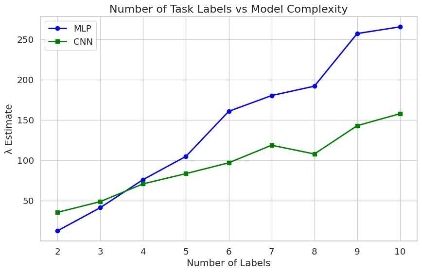
The results show a linear scaling law relating number of labels to task complexity. The CNN typically has a lower \hat{\lambda} than the MLP, which matches intuitions that some of the complexity is “stored” in the architecture because the convolutions apply a useful prior on functions good at solving image recognition tasks.
Is there any intuition or claim about why they look like they're only diverging after 5 classes/task-labels?
My first guess was that it's noise from the label ordering (some of the digits must be harder to learn than others). Ran it 10 times with the labels shuffled each time:
Still unsure.
If you're able to shift the crossover by just more resampling, yeah, that suggests that the slight inversion is a minor artifact - maybe the hyperparameters are slightly better tuned at the start for MLPs compared to CNNs or you don't have enough regularization for MLPs to keep them near the CNNs as you scale which exaggerates the difference (adding in regularization is often a key ingredient in MLP papers), something boring like that...
The local learning coefficent λ is a measure of a model's "effective dimensionality" that captures its complexity (more background here). Lau et al recently described a sampling method (SGLD) using noisy gradients to find a stochastic estimate ^λ in a computationally tractable way (good explanation here):
I present results (Github repo) of the "Task Variability" project suggested on the DevInterp project list. To see how degeneracy scales with task difficulty and model class, I trained a fully-connected MLP and a CNN (both with ~120k parameters) on nine MNIST variants with different subsets of the labels (just the labels {0, 1}, then {0, 1, 2}, etc.). All models were trained to convergence using the same number of training data points. I implement Lau et al's algorithm on each of the trained models. The results below are averaged over five runs:
The sampling method is finicky and sensitive to the hyperparameter choices of learning rate and noise factor. It will fail by producing negative or very high ^λ values if the noise ϵand the distance penalty γ (see lines 6 and 7 in the pseudocode above) isn't calibrated to the model's level of convergence. The results show a linear scaling law relating number of labels to task complexity. The CNN typically has a lower ^λ than the MLP, which matches intuitions that some of the complexity is "stored" in the architecture because the convolutions apply a useful prior on functions good at solving image recognition tasks.