I'm curious about your sense of the path towards AI safety applications, if you have a more specific and/or opinionated view than the conclusion/discussion section.
My main opinionated view relative to current discourse is that if someone is trying to apply any of this directly to LLMs, then they are probably very deeply confused about natural abstractions and also language and also agency/intelligence/etc in general.
The path we're optimizing for right now is to figure out the whole damn core of the theory of agency, get it across the theory-practice gap, and then not be so clueless about everything. See The Plan. Possibly with AI acceleration of the research at some point; our decisions right now are basically the same regardless of whether the research will be accelerated by AI later.
(Mediation)
Wait, so it's enough for the agents to just believe the observables are independent given the state of their latents? We only need the to be independent conditional on under a particular model ?
I didn't realise that. I thought the observables had to be 'actually independent' after conditioning in some sort of frequentist sense.
Getting a version of this that works under approximate Agreement on Observables sounds like it would be very powerful then. It'd mean that even if Alice is much smarter than Bob, with her model e.g. having more FLOP which she can use to squeeze more bits of information out of the data, there'd still need to be a mapping between the concepts Bob and Alice internally use in those domains where Bob doesn't do very much worse than Alice on predictive accuracy.
So, if a superintelligence isn't that much better than humanity at modelling some specific part of reality, there'd need to be an approximate mapping between humanity's latents and (some of) the superintelligence's latents for that part of reality. If the the theorems approximately hold under approximate agreement on observables.
Yup, that is correct.
If the the theorems approximately hold under approximate agreement on observables.
Yeah, there is still the issue that the theorems aren't always robust to approximation on the Agreement on Observables condition, though the Solomonoff version is and there's probably other ways to sidestep the issue.
I think a subtle point is that this is saying we merely have to assume predictive agreement of distributions marginalized over the latent variables , but once we assume that & the naturality conditions, then even as each agent receive more information about to update their distributions & latent variables , the deterministic constraints between the latents will continue to hold.
Or if a human and AI start out with predictive agreement over some future observables, & the AI's latent satisfy mediation while human's latent satisfy redundancy, then we could send the AI out to update on information about those future observables, and humans can (in principle) estimate the redundant latent variable they care about from the AI's latent without observing the observables themselves. The remaining challenge is that humans often care about things that are not approximately deterministic w.r.t observables from typical sensors.
Yes, though I'll flag that we don't have robustness with respect to approximation on the agreement condition (though we do have other ways around that to some extent, e.g. using the Solomonoff version of natural latents), and those sorts of updates are the kind of thing which I'd expect to run into that robustness problem.
...how is that a way around it? It looks to me like, there, you both for sure observe the same datapoints, even if you're allowed to condition on extra stuff by adding the additional length required to the epsilons.
Just skimmed for now...
We say a latent is a "redund" over observables if and only if is fully determined by each individually, i.e. there exist functions such that for each . In the approximate case, we weaken this condition to say that the entropy for all , for some approximation error .
I see your latest result has allowed you to streamline the definitions of redundancy and redunds.
I think attempting to require to be small in terms of would still run into my counterexample, right? (Setups could be constructed such that requiring to be -small would cause to scale arbitrarily with , and vice versa. So in the general case, there may exist valid redunds with the redundancy error such that the maximal redund's and (and therefore ) cannot both be -small.)
Graphical statement of Theorem 2
I find this picture pretty misleading, because it seems to say that if is determined by , then is a mediator, when really this is false, and it's stated explicitly in the text above that Alice's latent satisfying mediation is assumed.
I think you might have misread something? The graphical statement of theorem 2 does not say that if is determined by , then is a mediator; that would indeed be false in general. It says that:
- If is a mediator and we have agreement on observables, then...
- ... naturality of implies that is determined by .
In particular, the theorem says that under some conditions is determined by . Determination is in the conclusion, not the premises. On the flip side, being a mediator is in the premises, not the conclusion.
This was all clear to me, but only from reading the text; my comment is just to say that the graphical statement doesn't show being a mediator in the premises, so in isolation it gives the wrong idea; this led to a little confusion.
To be clear, I am talking about the reverse direction, as pictured here:
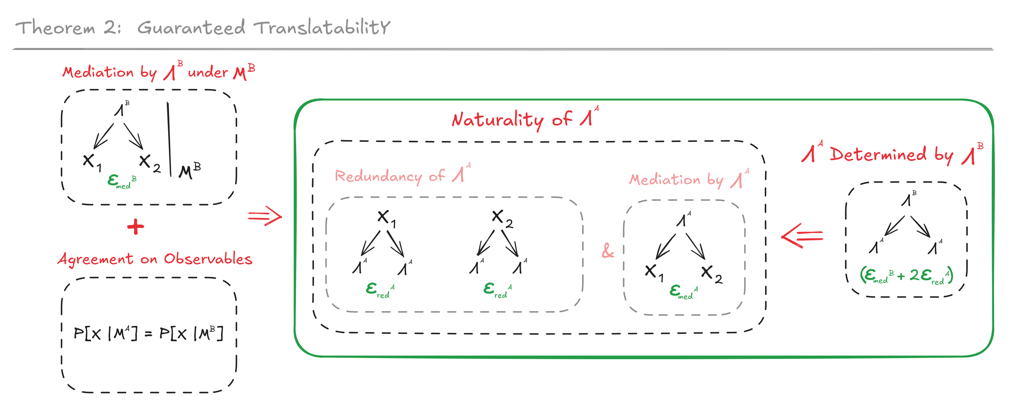
I understand that you have already set up as a mediator immediately above the image. Your text is perfectly clear:
In other words, we want to show: if Alice' latent satisfies Mediation, and for any latent Bob could choose (i.e. any other mediator) we have , then Alice' latent must be natural.
The other problem is that the image has only a single B, but the actual theorem proves necessity of Alice's being a redund from the requirement that hers is determined by all possible Bob's (that are mediators and agree on observables). Without the for all, you can't sub in X_1 and X_2 for his latent.
Which formal properties of the KL-divergence do the proofs of your result use? It could be useful to make them all explicit to help generalize to other divergences or metrics between probability distributions.
The appendices make heavy use of additivity across independent variables (and across factorizations more generally), which is the main thing I'd expect to need to work around in order to use other divergences/metrics.
Really gorgeous stuff with philosophically significant and plausibly practical implications. Great work. I assume you've also looked at this from a categorial perspective? It would surprise me if treating latents as limits didn't simplify some of the arguments (or at least the presentation, which is already admirably clear). And I can't help but wonder whether "bigger" uniqueness/isomorphism/stability results for world-models or other features of agents might result from comparing Bayes net categories. If you haven't tried categorial abstractions (I dunno the specifics---there are a few categorification choices that I could see being useful here), play around with them.
In case anyone's wondering: You really do have to assume Alice has a mediator for the necessity on the translation theorem. That is you can't derive it from being determined by all mediators - otherwise, her "latent" could be a constant. Intuitively: translation means that all her info is in all mediators that Bob could have, while the mediator condition is says she has "enough" info to be a natural latent instead of something stupid like a constant.
Exercise for the Reader: By separately tracking the
's on the two redundancy conditions through the proof, show that, for this example, the coin's true bias approximately mediates between the coinflips and Carol's median to within , i.e., roughly 0.058 bits.
(anyone reading this should try it themselves before reading my solution - it's immediate, you can probably do it).
To prove the mediator determines redund theorem, you apply dangly bits to each branch of the mediation diagram, each time using one of the redundancy conditions. Dangly Bits makes the errors add, so theorem really is
Graphical statement of Theorem 2
The image you want should look like this[1]:
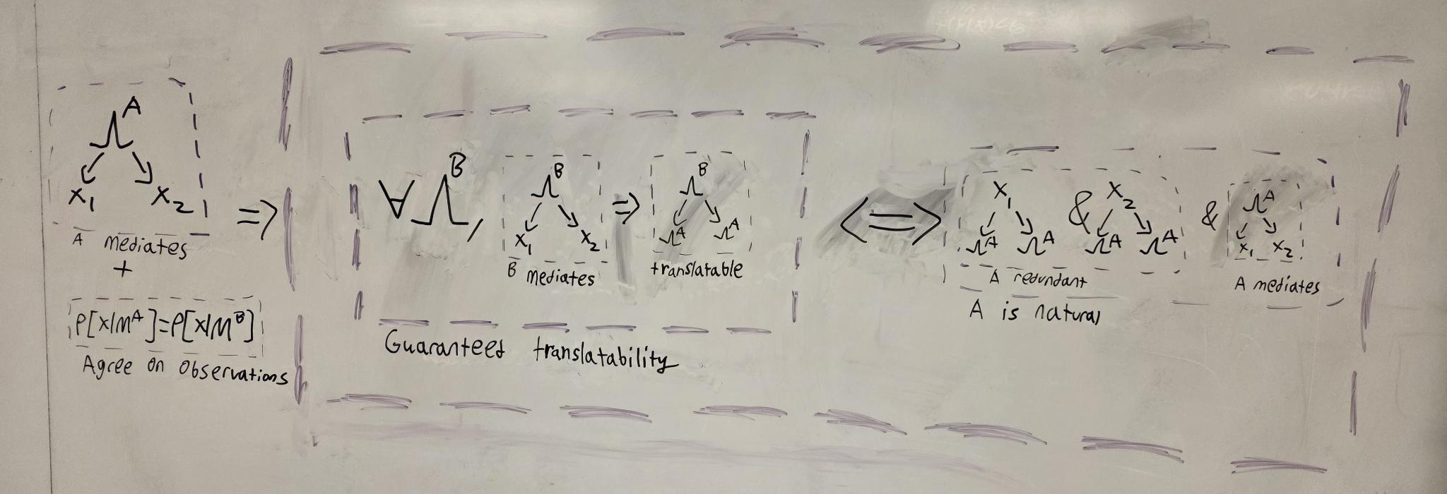
I think you have two errors in your picture (the text is fine).
My understanding from the text is that you have proven:
If Alice's latent is a mediator then (Alice's is a natural latent <-> (for all possible Bob's where Bob's latent is a mediator and Alice and Bob agree on observables, Bob's latent determines Alice's)
The image leaves out the bolded bits, namely it leaves out that
- Alice's latent is assumed to be a mediator
- The theorem is about what Alice needs to do to have a guarantee for all Bob's.
That is, the image says: Bob mediation + Alice and Bob agree on observables -> (Alice's is a natural latent <-> Bob's determines Alice's)
- ^
I didn't put the epsilons, and it'd easier to read if you swap the two parts of the conclusion in my image so that it's like yours. That is, it'd be easier if I said [A is natural] <-> [every B that mediates is translatable to A]
Great work! I have a technical question.
My current understanding is as follows:
1. If we have even one observable variable with agreement observation and for which the latent variables satisfy the exact naturality condition, we can then build the transferability function exactly.
2. In the approximation case, if we have multiple observable variables that meet these same conditions, we can choose the specific variable (or set of variables, in the proofs you used a couple) that will minimize the errors. We would not need to use all of them.
Is this correct?
Additionally, I was wondering if you have attempted to implement the algorithm derived from the proof to construct the isomorphism. It seems that some effort could be dedicated to developing an algorithm that minimizes or reduces these errors. It could one day be helpful for interpreting and aligning different ontological frameworks, like mapping an alien Bayesian network to a human one.
I do not understand the statement of your current understanding, in particular point 1. Could you please state in different words and/or state it formally and/or give an example?
By scanning the graphical proof, I don't see any issue on the following generalization of the Mediator Determines Redund Theorem:
Let and be random variables and let be any not-empty subset of that satisfy the following conditions:
- Mediation: are independent given
- Redundancy:
Then .
In the above, I've weaken the Redundancy hypothesis, requiring that the redundancy of any subset of random variables is enough to conclude the thesis.
Does the above generalization work (if don't, why?).
If the above stands true, then just one observational random variable (with agreement) is enough to satisfy the Redundancy condition (Mediation is trivially true with one variable), an therefore is determined by Moreover, in the general approximation case, if we have various sets of random variables that meet the naturality condition, we can choose the one that will minimize the errors (there's some kind of trade-off between and errors).
Ah, yes, that is almost correct. You need redundancy over TWO distinct observables (i.e. the subset must be at least size two), not just one, but otherwise yes. With just one observable, you don't have two branches to dangle a off of in the graphical proof, so we can't get between two copies of .
Background on where this post/paper came from
About a year ago, we wrote up a paper on natural latents for the ILLIAD proceedings. It was mediocre. The main shortcoming stemmed from using stochastic rather than deterministic natural latents, which give much less conceptually satisfying ontological stability guarantees; there was this ugly and confusing caveat on everything throughout the paper. We knew at the time that deterministic natural latents gave a much cleaner story, but we were more concerned about maintaining enough generality for our results to bind to reality than about getting the cleanest story.
Recently, we proved thatexistence of a stochastic natural latent implies existence of a deterministic natural latent(specifically under approximation; the exact case is easy). So now, we can write the paper the way we'd really like, without sacrificing generality.UPDATE: Nope, that proof turned out to have a fatal flaw, the problem is still open.This post is an overhaul of (and large improvement to) a paper we wrote about a year ago. The pdf version is available on arXiv here. As of posting, this is probably the best first-stop mathematical intro to natural latents.
Abstract
Suppose two Bayesian agents each learn a generative model of the same environment. We will assume the two have converged on the predictive distribution (i.e. distribution over some observables in the environment), but may have different generative models containing different latent variables. Under what conditions can one agent guarantee that their latents are a function of the other agent’s
latents?
We give simple conditions under which such translation is guaranteed to be possible: the natural latent conditions. We also show that, absent further constraints, these are the most general conditions under which translatability is guaranteed. Crucially for practical application, our theorems are robust to approximation error in the natural latent conditions.
Background
When is robust translation possible at all, between agents with potentially different internal concepts, like e.g. humans and AI, or humans from different cultures? Under what conditions are scientific concepts guaranteed to carry over to the ontologies of new theories, (e.g. as general relativity reduces to Newtonian gravity in the appropriate limit?) When and how can choices about which concepts to use in creating a scientific model be rigorously justified, like e.g. factor models in psychology? When and why might a wide variety of minds in the same environment converge to use (approximately) the same concept internally?
These sorts of questions all run into a problem of indeterminacy, as popularized by Quine[1]: Different models can make exactly the same falsifiable predictions about the world, yet use radically different internal structures.
On the other hand, in practice we see that
Combining those, we see ample empirical evidence of a high degree of convergence of internal concepts between different humans, between humans and AI, and between different AI systems. So in practice, it seems like convergence of internal concepts is not only possible, but in fact the default outcome to at least a large extent.
Yet despite the ubiquitous convergence of concepts in practice, we lack the mathematical foundations to provide robust guarantees of convergence. What properties might a scientist aim for in their models, to ensure that their models are compatible with as-yet-unknown future paradigms? What properties might an AI require in its internal concepts, to guarantee faithful translatability to or from humans' concepts?
In this paper, we'll present a mathematical foundation for addressing such questions.
The Math
Setup & Objective
We'll assume that two Bayesian agents, Alice and Bob, each learn a probabilistic generative model,
However, the two generative models may use completely different latent variables
Crucially, we will assume that the agents can agree (or converge) on some way to break up X into individual observables
We require that the latents of each agent's model fully explain the interactions between the individual observables, as one would typically aim for when building a generative model. Mathematically,⫫
Given that Alice' and Bob's generative models satisfy these constraints (Agreement on Observables and Mediation), we'd like necessary and sufficient conditions under which Alice can guarantee that her latent is a function of Bob's latent. In other words, we'd like necessary and sufficient conditions under which Alice' latent
We will show that:
Notation
Throughout the paper, we will use the graphical notation of Bayes nets for equations. While our notation technically matches the standard usage in e.g. Pearl[5], we will rely on some subtleties which can be confusing. We will walk through the interpretation of the graph for the Mediation condition to illustrate.
The Mediation condition is shown graphically below.
The graph is interpreted as an equation stating that the distribution over the variables factors according to the graph - in this case,
Besides allowing for compact presentation of equations and proofs, the graphical notation also makes it easy to extend our results to the approximate case. When the graph is interpreted as an approximation, we write it with an approximation error
In general, we say that a distribution
We'll also use a slightly unusual notation to indicate that one variable is a deterministic function of another:
Foundational Concepts: Mediation, Redundancy & Naturality
Mediation and redundancy are the two main foundational conditions which we'll work with.
Readers are hopefully already familiar with mediation. We say a latent
Redundancy is probably less familiar, especially the definition used here. We say a latent
Intuitively, all information about
We'll be particularly interested in cases where a single latent is both a mediator and a redund over
Justification of the name "natural latent" is the central purpose of this paper: roughly speaking, we wish to show that natural latents guarantee translatability, and that (absent further constraints) they are the only latents which guarantee translatability.
Core Theorems
We'll now present our core theorems. The next section will explain how these theorems apply to our motivating problem of translatability of latents across agents; readers more interested in applications and concepts than derivations should skip to the next section. We will state these theorems for generic latents
Theorem: Mediator Determines Redund
Suppose that random variables
Then
In English: if one latent
The graphical statement of the Mediator Determines Redund Theorem is shown below, including approximation errors. The proof is given in the Appendix.
The intuition behind the theorem is easiest to see when
Naturality
We're now ready for the corollaries which we'll apply to translatability in the next section.
Suppose a latent
Naturality
There is also a simple dual to "Naturality
Isomorphism of Natural Latents
If two latents
In the approximate case, each latent has bounded entropy given the other; in that sense they are approximately isomorphic.
Application To Translatability
Motivating Question
Our main motivating question is: under what conditions on Alice' model
Recall that we already have some restrictions on Bob's model and latent(s): Agreement on Observables says
Since Naturality
Guaranteed Translatability
If Alice' latent
Now it's time for the other half of our main theorem: the naturality conditions are the only way for Alice to achieve this guarantee. In other words, we want to show: if Alice' latent
The key to the proof is then to notice that
Alice' latent already had to satisfy the mediation condition by assumption, it must also satisfy the redundancy condition in order to achieve the desired guarantee, therefore it must be a natural latent. And if we weaken the conditions to allow approximation, then Alice' latent must be an approximate natural latent.
In English, the assumptions required for the theorem are:
Under those constraints, Alice can guarantee that her latent
Proof: the "if" part is just Naturality
Natural Latents: Intuition & Examples
Having motivated the natural latent conditions as exactly those conditions which guarantee translatability, we move on to building some intuition for what natural latents look like and when they exist.
When Do Natural Latents Exist? Some Intuition From The Exact Case
For a given distribution
Let's suppose that there are just two observables
This is a deterministic constraint between
Next, the mediation condition. The mediation condition says that
On the other hand, if
That gives us an intuitive characterization of the existence conditions for exact natural latents: an exact natural latent between two (or more) variables exists if-and-only-if the variables are independent given the value of a deterministic constraint across those variables.
Worked Quantitative Example of the Mediator Determines Redund Theorem
Consider Carol who is about to flip a biased coin she models as having some bias
Intuitively, if the bias
The Mediator Determines Redund Theorem, then tells us that the bias approximately mediates between the median (computed from either batch) and the coinflips
This is a Dirichlet-multinomial distribution, so it is cleaner to rewrite in terms of
Writing out the distribution and simplifying the gamma functions, we obtain:
There are only
Returning to the Mediator Determines Redund Theorem, we have
Exercise for the Reader: By separately tracking the
Intuitive Examples of Natural Latents
This section will contain no formalism, but will instead walk through a few examples in which one would intuitively expect to find a nontrivial natural latent, in order to help build some intuition for the reader. The When Do Natural Latents Exist? section provides the foundations for the intuitions of this section.
Ideal Gas
Consider an equilibrium ideal gas in a fixed container, through a Bayesian lens. Prior to observing the gas, we might have some uncertainty over temperature. But we can obtain a very precise estimate of the temperature by measuring any one mesoscopic chunk of the gas. That's an approximate deterministic constraint between the low-level states of all the mesoscopic chunks of the gas: with probability close to 1, they approximately all yield approximately the same temperature estimate.
Due to chaos, we also expect that the low-level state of mesoscopic chunks which are not too close together spatially are approximately independent given the temperature.
So, we have a system in which the low-level states of lots of different mesoscopic chunks are approximately independent given the value of an approximate deterministic constraint (temperature) between them. Intuitively, those are the conditions under which we expect to find a nontrivial natural latent. In this case, we expect the natural latent to be approximately (isomorphic to) temperature.
Biased Die
Consider 1000 rolls of a die of unknown bias. Any 999 of the rolls will yield approximately the same estimate of the bias. That's (approximately) the redundancy condition for the bias.
We also expect that the 1000 rolls are independent given the bias. That's the mediation condition. So, we expect the bias is an approximate natural latent over the rolls.
However, the approximation error bound in this case is quite poor, since our proven error bound scales with the number
Timescale Separation In A Markov Chain
In a Markov Chain, timescale separation occurs when there is some timescale
Discussion & Conclusion
We began by asking when one agent's latent can be guaranteed to be expressible in terms of another agent's latent(s), given that the two agree on predictions about two observables. We've shown that:
...for a specific broad class of possibilities for the other agent's latent(s). In particular, the other agent can use any latent(s) which fully explain the interactions between the two observables. So long as the other agent's latent(s) are in that class, the first agent can guarantee that their latent can be expressed in terms of the second's exactly when the natural latent conditions are satisfied.
These results provide a potentially powerful tool for many of the questions posed at the beginning.
When is robust translation possible at all, between agents with potentially different internal concepts, like e.g. humans and AI, or humans from different cultures? Insofar as the agents make the same predictions about two parts of the world, and both their latent concepts induce independence between those parts of the world (including approximately), either agent can ensure robust translatability into the other agent's ontology by using a natural latent. In particular, if the agents are trying to communicate, they can look for parts of the world over which natural latents exist, and use words to denote those natural latents; the equivalence of natural latents will ensure translatability in principle, though the agents still need to do the hard work of figuring out which words refer to natural latents over which parts of the world.
Under what conditions are scientific concepts guaranteed to carry over to the ontologies of new theories, like how e.g. general relativity has to reduce to Newtonian gravity in the appropriate limit? Insofar as the old theory correctly predicted two parts of the world, and the new theory introduces latents to explain all the interactions between those parts of the world, the old theorist can guarantee forward-compatibility by working with natural latents over the relevant parts of the world. This allows scientists a potential way to check that their work is likely to carry forward into as-yet-unknown future paradigms.
When and why might a wide variety of minds in the same environment converge to use (approximately) the same concept internally? While this question wasn't the main focus of this paper, both the minimality and maximality conditions suggest that natural latents (when they exist) will often be convergently used by a variety of optimized systems. For minimality: the natural latent is the minimal variable which mediates between observables, so we should intuitively expect that systems which need to predict some observables from others and are bandwidth-limited somewhere in that process will often tend to represent natural latents as intermediates. For maximality: the natural latent is the maximal variable which is redundantly represented, so we should intuitively expect that systems which need to reason in ways robust to individual inputs will often tend to track natural latents.
The natural latent conditions are a first step toward all these threads. Most importantly, they offer any mathematical foothold at all on such conceptually-fraught problems. We hope that foothold will both provide a foundation for others to build upon in tackling such challenges both theoretically and empirically, and inspire others to find their own footholds, having seen that it can be done at all.
Acknowledgements
We thank the Long Term Future Fund and the Survival and Flourishing Fund for funding this work.
Appendices
Graphical Notation and Some Rules for Graphical Proofs
In this paper, we use the diagrammatic notation of Bayes networks (Bayes nets) to concisely state properties of probability distributions. Unlike the typical use of Bayes nets, where the diagrams are used to define a distribution, we assume that the joint distribution is given and use the diagrams to express properties of the distribution.
Specifically, we say that a distribution
Frankenstein Rule
Statement
Let
More generally, if
We'll prove the approximate version, then the exact version follows trivially.
Proof
Without loss of generality, assume the order of variables respected by all original diagrams is
The proof starts by applying the chain rule to the
=
Then, we add a few more expected KL-divergences (i.e., add some non-negative numbers) to get:
=
Thus, we have
Factorization Transfer
Statement
Let
then
where
Proof
As with the Frankenstein rule, we start by splitting our
Next, we subtract some more
Thus, we have
Bookkeeping Rule
Statement
If all distributions which exactly factor over Bayes net
Proof
Let
Now, we have:
Thus:
By the Factorization Transfer Theorem, we have:
which completes the proof.
The Dangly Bit Lemma
Statement
If
Proof
Let
Graphical Proofs
Python Script for Computing
W. V. O. Quine, On empirically equivalent systems of the world, Erkenntnis 9, 313 (1975).
H. Cunningham, A. Ewart, L. Riggs, R. Huben, and L. Sharkey, Sparse autoencoders find highly interpretable features in
language models, (2023), arXiv:2309.08600 [cs.LG].
Marvik, Model merging: Combining different fine-tuned LLMs, Blog post (2024), retrieved from https://marvik.com/
model-merging.
M. Huh, B. Cheung, T. Wang, and P. Isola, The platonic representation hypothesis, (2024), arXiv:2405.07987 [cs.LG].
J. Pearl, Causality: Models, Reasoning and Inference, 2nd ed. (Cambridge University Press, USA, 2009).