As we all know, any sufficiently-advanced technology is indistinguishable from magic. Accordingly, whenever such artifact appears, a crowd of researchers soon gathers around it, hoping to translate the magic into human-understandable mechanisms, and perhaps gain a few magical powers in the process.
Traditionally, our main supply of magical technology to study came from mysterious entities called "biological organisms", and the task of figuring how they work fell to a sect of mages called the "molecular biologists".
Recently, however, a new category of entities called "large language models" came into the spotlight, and soon a new guild of mages, the "mechanistic interpretability researchers", spawned around it. Their project: to crack open the black box of AI and reveal the mechanisms inside.
However, their task is a bit different from molecular biology. First, LLMs are large. The largest models to date contain more than a trillion floating-point parameters. As a rough point of comparison, the human genome is encoded by only 3.1 billion nucleotides. These things aren't exactly commensurable, but it goes to say LLMs have room to store quite a lot of mechanisms, and potentially very complicated ones.
Second, LLMs are changing all the time. As of 2025, AI models are now casually demolishing International Math Olympiad problems. Meanwhile, some clever work from earlier this year revealed how a small model from 2021 performs addition. There is even some tentative evidence about multiplication. But ask how LLMs solve a first-order equation, and we're back to magic.
Therefore, one thing is clear: if we want the slightest chance at reading the minds of our robots, we'll have to find a way to dramatically scale up the scientific method.
One recent approach to do this is called parameter-space decomposition (PD). PD claims that it’s possible to take a neural network, and automatically break it down into all the elementary mechanisms it contains. If we can make this work, it will give us an exploded view of the whole neural network, allowing to track down the flow of information through the system and make precise predictions about its behavior.
like this but the motorcycle engine is general superintelligence
This post is meant as an intuitive explanation of parameter-space decomposition. I'll go over the points I found the most confusing, and I will do my best to deconfuse them. I expect this to be useful to:
People who want to get into this kind of research
People worried about the future of humanity, who want to make up their own mind about whether interpretability has a chance to succeed at making AI safer
People curious about the conceptual questions – how do you define a mechanism in practice? How would you extract meaningful knowledge from a giant organism you know nothing about, if you could automatically perform hundreds of thousands of experiments over the night?
For this post, I'll focus on the latest iteration of PD, as described in the paper by Bushnaq et al., 2025: Stochastic Parameter Decomposition (SPD). It doesn't require much background knowledge, but you should have at least some vague familiarity with neural networks.
The parameter-space decomposition project
First, we need to put things back in their historical context. So far, much of the attempts at figuring out what a neural network is doing at scale have relied on inspecting the neuron activations: which neurons are active, and how much. This is, in a sense, an attempt to inspect how the network "represents" information – if we carefully record the activations while we expose the network to a lot of discourse about bananas, there’s good hope we can identify some recognizable banana pattern, and now you can tell when the network is thinking about bananas.
Extending and refining this basic idea, we get the activation-space interpretability project: not just identifying features, but also tracking down how they relate to each other, and how having some feature somewhere in the network leads to some other features popping up in some other place. This approach has given promising results, and people have been drawing maps of increasingly large networks this way.
Enter parameter-space interpretability. Instead of explaining the behavior of the network in terms of activation features, we want to break it down into mechanisms, where each mechanism is itself structured like a "little neural network" with its own weights, describing a specific part of the network's calculations. These mechanisms, taken all together, should recapitulate the behavior of the whole network. They should also allow to identify a minimal set of mechanisms responsible for processing any given forward pass, so it can be inspected and understood in isolation.
How can we possibly achieve that?
A scalable definition of "mechanism"
Mechanisms are often defined in relation to a specific task. For example, if you have a bicycle and you want to know how the braking works, you could try removing various parts of the bicycle one by one, and every time check if the bike can still brake. Eventually, you'll find a list of all the little parts that are involved in braking, and cluster these parts together as "the braking mechanism".
Unfortunately, this is not a scalable definition: remember, our end goal is to identify every single mechanism in a gargantuan neural network, all at once. We can't afford to investigate each task one by one – in fact, we don't even know what the tasks are!
What we have, though, is the original training data. This means that we can put the network back in all the situations it was trained to process. We will take advantage of this to define mechanisms in a much more scalable way.
As an analogy, imagine we are trying to completely "decompose" a bicycle. We could proceed as follows:
Break down the bicycle into little "building blocks", that can be removed independently to see if they are important in a given situation
Iterate over every possible situation in the bicycle's life cycle. For each situation, remove each of the parts one by one, and write down which parts have an effect on the bike's behavior or not
Red = active, black = inactive
Take all the building blocks that influence the bike's behavior in the exact same subset of situations, and cluster them together as "the same mechanism". If your collection of situations is fine-grained enough, this should roughly correspond to parts that "perform the same task".
This is, in essence, what we are going to do with our neural network. Before we can actually do this, we need to clarify two things:
What does it mean to break down a neural network into "building blocks"? What's an "elementary building block" of neural network?
What does it mean to "remove" a part, concretely?
An atom of neural network computation
Neural networks are often depicted as little circles connected by little lines, but, under the hood, it’s all matrix multiplication. This is usually how they are implemented in practice:
Take the neuron activations of the first layer, and write them in order as a vector x. Each entry of the weight matrix Mi,j represents the weight between neuron i of the first layer and neuron j in the next layer. The activation of the second layer are then Mx, plus some bias b.
This will be our starting point: a big neural network full of matrices.
We need to decompose the matrices into basic buildings blocks, such that:
Any mechanism in the network can be described using in terms of these building blocks (assembling several together as needed)
If we take all the building blocks and put them together, we get the original network
A naive choice would be to use individual matrix entries as building blocks, but this falls apart very quickly: neuralnetworksdistributetheir calculations over many neurons, using representations that are usually not aligned to the neuron basis, such that a single weight will almost always be involved in all kinds of unrelated operations.
What SPD does is split each matrix into a stack of many rank-1 matrices, whose values sum up exactly to the original weights.
These rank-1 matrices, called subcomponents, are what we will use as our fundamental building blocks. As we'll see, rank-1 matrices are a great candidate for an "atom" of neural-network computation:
We can describe a wide variety of mechanisms by combining just a few of them
We can "ablate" them from the network, and see if this has an effect on the network's behavior on any given input
Let's examine more closely what they do.
By definition, a rank-1 matrix can be written as the outer product of two vectors, that I’ll call Vout and Vin:
The geometric interpretation is that it recognizes a direction Vin in the input (by taking the dot product VTin⋅x, resulting in a scalar value), and writes the same amount to the Vout direction in output space. In the context of a neural network, one could say Vin detects a "feature" in the previous layer's activations, and writes another feature Vout to the next layer in response.
(In real-life, this happens in spaces with tens of thousands of dimensions, so x, Vin and Vout can all contain a lot of information. They might correspond to something like “a complete description of Michael Jordan”.)
What rank-1 matrices can and cannot do
What makes rank-1 matrices great as "atoms of computation" is that they are quite expressive, and at the same time very restricted.
They are expressive, because they can basically read any feature, and write any other feature in response. This is enough to implement a lot of the basic computation that is rumored to occur in LLMs. For example, the following actions would be easy to express in terms of rank-1 matrices:
In a transformer's attention layer, the query matrix recognizes a trigger feature, and writes a signal out. Somewhere else, the key matrix recognizes another trigger feature, and writes the same signal. The two “recognize” each other in the attention pattern, then the value/output matrices write some relevant data to the residual stream, to be used by downstream layers
In a multi-layer perceptron, the first layer recognizes a feature in the residual stream, and activates the corresponding hidden neuron. In return, the second layer of the perceptron adds relevant memorized data to the residual stream.
If we could identify this kind of basic operations inside LLMs, that would already be a big step forward for interpretability.
But rank-1 matrices are also restricted:
Whatever happens, they can only write in the direction of Vout. No matter what obscure adversarial fucked-up OOD input you feed it, the space of possible outputs is just limited mathematically to that one direction.
Similarly, the amplitude of the outcome is entirely encapsulated by the dot product between the input and Vin.
In other words, if your network is completely decomposed into a finite set of rank-1 subcomponents, you can set some strict mathematical boundaries on what can possibly happen.
Combining rank-1 matrices to make higher-rank components
Importantly, we are not assuming that all mechanisms are made exclusively of rank-1 transformations. Since our building blocks are all matrices the same size as the original, we can add several of them to build higher rank matrices – n of them for a rank-n transformation. This ability to combine the building blocks together to form more complex mechanisms is in fact a distinguishing feature of PD compared to current activation space methods like transcoders.
For example, imagine that a network represents the time of the day as the angle of a vector within a 2D plane – pretty much like the hand of a clock. Then, imagine there is a "3 hours later" mechanism that just rotates this vector by 45° within the plane. In parameter-space, this can be performed by a 2D rotation matrix. This is a rank-2 operation, so it can just be written as the sum of two rank-1 matrices, with orthogonal input vectors.
Meanwhile, it would be really difficult to account for this using classic activation-space methods: a classic transcoder would try to make a feature for each possible time of the day, and map each of them to its "3h later" counterpart. That wouldn't be very accurate, and much harder for us to interpret than the rotation explanation.
And rotations are, of course, only one particular case of higher-rank transformation. They are probably commonplace in large neural networks – for example, to performoperations on numbers stored on an helical structure, or when dealing with positional embeddings. All sorts of other exotic feature geometries are possible in principle. So, having access to the actual matrices that generate and transform the features would be a pretty big deal.
Carving out the subcomponents
Of course, there are infinitely many ways to split a high-rank matrix into a sum of rank-1 components. Here comes the difficult part: how do we split the original matrices into rank-1 components that accurately describe the calculations of the network?
To do this, we need to make a central assumption: any given input will be processed by a small subset of the available mechanisms. For example, predicting the weather and translating Ancient Greek should rely on two quite different sets of mechanisms. For general-purpose large language models, this sounds a priori reasonable: provided there's a mechanism that links "Michael Jordan" to "basketball", it's probably inactive for the vast majority of inputs.
If this assumption is true, then there is hope we can tease out the "correct" subcomponents: we want to split our original matrices into a collection of rank-1 subcomponents, such we can recreate the behavior of the model on any input, using only a small selection of them each time. Specifically, on any given input, we want to be able to ablate as many subcomponents as possible, without changing the output.[1]
To better understand what this means, let's consider what happens mechanistically when you "ablate" a rank-1 subcomponent from a neural network matrix.
Surgically removing unnecessary computation
Remember that we want our subcomponents to sum up to the original weights:
Woriginal=∑iVout,iVTin,i
where i is the index of the subcomponent.
Ablating a subcomponent simply means that, when taking the sum, we set this subcomponent to zero. Furthermore, we can ablate a subcomponent partially by multiplying it by some masking coefficient m between 0 and 1. We just replace each matrix in the network with a masked version:
Wablated=∑imiVout,iVTin,i
Now we can run the masked network, and check whether it still produces the same output as the original version.
How does that work in practice? Remember, the subcomponents are rank-1 matrices. So there are two clear cases where ablation should be possible:
The input feature Vin is absent from the previous layer’s activations. If VTinx=0 then VoutVTinx will always be zero, and ablating the subcomponent will have no effect.
Moving the next layer’s activations in the Vout direction has no downstream effect (at least in the [0,VTinx]) interval. This could be for a variety of reason, for example:
This subcomponent is part of the Q matrix of a transformer’s attention mechanism, and there is no corresponding feature generated by the K matrix for this input
There's a deep cascade of downstream mechanisms that gradually erase the effect until it vanishes
To put it another way, when we ablate a subcomponent, weremove the connection between Vin and Vout. If the output of the network remains the same, then we can say that this connection didn’t participatein creating the output.
Let's look at a concrete example: let's decompose a simple little toy network called the toy model of superposition (TMS). As we'll see, despite being a toy model, it's a great illustration for many key concepts in parameter-space decomposition.
The TMS has an input layer with 5 dimensions, then a hidden layer with 2 dimensions, then an output layer with 5 dimensions again. This is followed by a ReLU activation. The input data is sparse (that is, most of the inputs will be zero everywhere except for 1 dimension), and the model is trained to reconstruct its inputs:
After training, here is what the TMS does to the data, when we feed it "one-hot" sparse inputs:
So, the inputs get compressed as 2D features in the hidden layer (arranged as the vertices of a pentagon in the 2D plane), then expanded back to 5D in the output layer. Expanding from 2D to 5D creates interference – the negative blue values in pre-ReLU outputs. But these are eliminated by the ReLU, and we end up with something similar to the inputs.
First, let's see how the first matrix, the one that takes sparse 5D inputs and compresses them into 2D, can be decomposed.
This is a rank-2 matrix, so in principle we could just write it as the sum of 2 subcomponents. But most inputs would then require both of them to be active at the same time.
Instead, there is a better way: make 5 subcomponents that each map one input to the associated 2D representation. In that case, the 5 Vinwould form an orthogonal basis: for each sparse input, we then have 1 subcomponent whose Vin is aligned to the input x, and 4 subcomponents for which Vinx=0. These 4 subcomponents can therefore be perfectly ablated without changing the output. As this allows to process most inputs using only 1 component, it is the preferred solution.
Now, let's see how we can decompose the second matrix.
We could, again, make 5 subcomponents using the 5 hidden features as their Vin. However, this time, the 5 hidden features are no longer orthogonal: the dot product of each feature with the Vin associated with the other features is not zero.
What makes it possible to decompose the second matrix is the ReLU nonlinearity: as it erases negative values, it also erases the interference produced by inactive subcomponents, making it possible to ablate them without changing the output.[2]
Thus, for the TMS, we can define these five elementary mechanisms, that sum up to the original weights:
This is an important example of how PD is able to accommodate features in superposition, by having more subcomponents than the rank of the matrix.[3]
(And this is indeed what the SPD algorithm finds. How does it get to this result? We'll jump into that later.)
Would things work this way in the context of a larger model? In general, for decomposition to be possible, either the features processed by a given matrix must be orthogonal enough that they can be ablated independently, or there must be something downstream that eliminates the interference between them. Arguably, these are reasonable things to expect – otherwise, the neural network wouldn't work very well in the first place.
An example of higher-rank mechanism
The TMS basically fits into the "linear representation" paradigm: each "feature" corresponds to a direction in activation-space, and the matrices are just reading and writing these features linearly. But, as we've seen above for rotation matrices, some mechanisms might work in a different way. What does the decomposition look like in that case?
The SPD paper includes a nice example of that. It is a slightly-modified version of the TMS above, but with an additional identity matrix inserted in between the two layers. This seems innocuous (the identity matrix does literally nothing), but it’s a great case study for how PD handles higher-rank mechanisms.
The 2×2 identity matrix has rank 2. Inside the TMS, it receives 5 different features, and must return each of them unchanged. What does the decomposition look like?
In the SPD paper, the 2×2 identity matrix is decomposed into these two subcomponents:
What are we looking at? Actually, this particular choice of 2 subcomponents is not particularly meaningful. What matters is that the off-diagonal elements cancel each other out, so these two subcomponents add up to the 2×2 identity matrix.
In practice, we would then notice that these two subcomponents always activate on the exact same inputs (in this case, every single input), cluster them together, and recover the identity matrix as our final mechanism.
The key point is that PD is able to encode higher-rank transformations, in a way that would be very difficult to capture using sparse dictionary learning on neuron activations.
Summoning the decomposed model
Now we have a clear idea of what the decomposed form of the network may look like, we can finally talk about the decomposition algorithm: how do we discover the correct decomposition, starting from the network's original weights?
The short answer is – gradient descent. At this point, we have some clear constraints about what subcomponents should look like. So the next step is simply to translate these constraints into differentiable loss functions, and train a decomposition model so that it satisfies all the conditions at once. We'll just initialize a bunch of random subcomponents for each matrix, then optimize them until they meet our requirements.
Let's recapitulate the constraints we are working with. There are 3 of them:
The weight faithfulness criterion: the subcomponents should add up to the original weights
The reconstruction criterion: on a given input, it should be possible to ablate the inactive subcomponents, and we should still obtain the same output
The minimality criterion: processing each input from the training data should require as few active subcomponents as possible
Let's see how each of these criteria are enforced in practice.
1. The weight faithfulness loss
This is simply the mean squared error between the original weights and the sum of the subcomponents. Weight faithfulness anchors the decomposed model to the original – it ensures that the mechanisms we discover actually correspond to what goes on in the original, and not something completely different that just happens to behave in the same way.
2. The stochastic reconstruction loss
For any input in the training data, we want to remove the inactive components, calculate the ablated model's output, and compare it to the original output. To do that, we first need a way to know which components are supposed to be active or not.
In SPD, this is done by attaching a tiny multi-layer perceptron (MLP) to every single candidate subcomponent. These MLPs are trained along the rest of the decomposition, and their task it to estimate by what fraction (from 0 to 1) their associated subcomponent can be safely ablated on the current input. They basically look at the previous layer's activations and say, "hmmm, dare I propose we ablate to as much as 0.3?". If the estimate is too low and the output changes, the MLP will get training signal so the fraction will be higher next time. This fraction is known as the causal importance, g(x).[4]
During decomposition, as the candidate subcomponents are still taking shape, the causal importance values will be somewhere between 0 and 1 – the imperfect subcomponents can be removed to some extent, but not totally. As the decomposition progresses, we hope for them to converge to either 1 (for active components) or 0 (for inactive ones).
After calculating the causal importances g(x) for each component, we can generate an ablated model with all components ablated as much as possible, and check that its output is still the same as the original – e.g., by taking the MSE or KL-divergence between the two.
Straightforward enough? Things are unfortunately more complicated. In fact, during decomposition, we don't completely ablate the inactive subcomponents as much as possible. We ablate them stochastically, to a randomly-chosen level between g(x) and 1. I'll explain why this is necessary in the next section.
3. The minimality loss
Remember, we are trying to find subcomponents such that as many of them as possible can be ablated on any given input.
The minimality loss is then simply defined as the sum of all causal importances g(x) over all candidate subcomponents for the current input (with an optional exponent). In other words, we are incentivizing the MLPs that calculate causal importances to output lower values whenever they can.
Here's how I picture what's happening: as training proceeds, the minimality loss pushes MLPs to predict lower and lower causal importances. But the imperfect subcomponents can only be ablated partially, not totally. This creates an error in stochastic reconstruction, which gets back-propagated to the subcomponents themselves, gradually aligning them to the correct directions.
this analogy is perfect and I will not elaborate
The important bit is that the minimality loss is the only loss we don't want to optimize too much: while we are aiming for perfect faithfulness and reconstruction, we want the subcomponents to be ablated just as much as they can bewithout compromising the other losses.
Accordingly, the minimality loss is usually multiplied by some very low coefficient – just what it takes to carve out the subcomponents, but not enough to distort them.
Why is stochastic parameter decomposition stochastic?
Why don't we just ablate the candidate subcomponents as much as we can?
The problem is, if we did that, the decomposed model wouldn’t necessarily reflect the true model. Instead, it would come up with components that perform the same operations as the original model, but implemented differently – possibly leveraging the causal-importance MLPs for extra flexibility.
Of course, these fake components wouldn’t add up to the original weights, but there’s a way around this: the decomposition could cheat by adding dead “filler” components, that are never active, but whose values fill up the difference between the fake weights and the real ones.
Let’s look at a concrete (fictional) example. Recall the 2×2 identity matrix above. A correct way to decompose it would be to use two rank-1 subcomponents, that each return one direction of the input space without changing it:
But here is an alternate decomposition: you could have multiple subcomponents, arranged in a circle. Then, we use the causal-importance MLPs to activate only the components that are aligned with the input activations. (For example, if the input is aligned with the red arrow, only the red arrow would be active and the rest would be ablated).
(Dead components are not shown)
This gives approximately the same result, except this time you need only 1 active subcomponent per input, instead of 2 for the true decomposition. So this fake decomposition would be favored over the correct one.
Now, consider what happens if we use stochastic reconstruction. Instead of ablating the components to their estimated causal importance g(x), they get ablated by a random fraction between g(x) and 1. We are asking for the model's output to remain the same for any point in the hyper-rectangle between "not-ablated-at-all" and "ablated-as-much-as-can-be":
a sketch with only 2 candidate subcomponents A and B
This means that even components that are fully inactive will be forced to activate randomly from time to time. This causes the cheating model to give incorrect outputs:
In other words, the cheating problem occurs because the decomposition exploits the power of the causal-importance MLPs to perform computation. We don’t want this – the causal-importance MLPs are just tools for deciding which components can be ablated! So the role of the stochastic reconstruction is basically to stop the decomposition model from relying on the causal-importance MLPs by making ablation non-deterministic, thus unreliable.[5]
In addition, stochastic activation prevents the model from filling up the target weights using arbitrary dead components – as the dead components get randomly activated too, they would interfere with the outputs. In practice, this means that the decomposition generates just enough subcomponents to replicate the model's behavior, and the remaining available subcomponents gets crushed to zero.
And yes, this is important enough for the whole method to be called "stochastic parameter decomposition".
What is parameter decomposition good for?
Now that we have a good sense of what the mechanisms look like and their properties, it's time to daydream about future applications. What can you do once you have a fully decomposed model? Does it make the robot apocalypse less likely? Can we finally get rid of the mechanism that makes Claude say "you're absolutely right to question this"?
Explaining the model's behavior
The nice thing about parameter-space components is that they give you a clean, closed-form formula for how the model calculated its answer. So you could, in principle, track down all the information that had a causal role in the model's decision.
After decomposing the model into subcomponents, the next step is to cluster the subcomponents that "work together" into larger mechanisms. These mechanisms may span multiple matrices and possibly implement some quite sophisticated algorithms, and I'm very curious about what kind of things we will find.[6]
To be clear, PD is only capable of identifying mechanisms at the tiniest level of organization. It is not meant to tell you everything you need to know about the model, but merely to find which elementary calculations the system is built upon. It’s shamelessly reductionist. I have no doubt that meaningful mechanisms exist at a higher level of organization (how the system plans, how it stores vocabularies for different human languages…) and breaking these down in rank-1 matrices will probably not be very illuminating. I still think it's plausible that understanding the lowest levels of organization is useful to understand higher mechanisms – if anything, as a scaffold to design experiments about them, in the same way progress in chemistry unlocked a lot of possibilities for biology.
Eliciting/editing the model's knowledge
One area where PD holds great promise is to access the information memorized by the model. It's not clear how LLMs store information in general, but there is good hope that we can identify which components represent specific facts about the world.
This could be extremely valuable, as it would enable you to know what knowledge about the world your robot is using at any given time – e.g., whether it's thinking about loopholes in the Geneva Convention when you ask for a cupcake recipe.[7]
The fact that inactive components can (by definition) be ablated when they are not active means that we can readily zero out the components we want the machine to forget (e.g., bio-weapons, British English, ...) while preserving the original behavior on all the other tasks.
Another approach would be to identify the minimal set of components that are necessary to process a narrow task, and use that to build an hyper-specialized model equipped only with these components, while being unable to do anything else.
Making experiments more tractable
Of course, this is all speculation. So far, PD has mostly been tested on tiny toy models, and people are only starting to scale it up to more realistic cases. There are many things that could go wrong and many assumptions that might not turn out to be true.
I think what makes parameter-space decomposition uniquely exciting is that it makes precise mathematical claims about what the model is doing. So, even if we don't know how well it will perform on real models, a big promise of PD is to narrow down the space of possible hypotheses about how the model works.
Once we know the Vin and Vout of all the components, we can make precise predictions about how the network will behave, why it behaves this way, and what could have caused it to behave otherwise. The point is not that these predictions will always be correct – the point is that, when they are not, it should be relatively straightforward to pinpoint where the discrepancy comes from.
For instance, if you claim you can scrape all mechanisms related to resiniferatoxin off an LLM, it should be relatively straightforward to inspect the actual effects of those mechanisms and investigate anomalies. This sounds more tractable than painting an anti-resiniferatoxin steering vector over the neuron activations, for which the mechanistic effect of the intervention is much more opaque.
Open questions
Finally, here is a sample of open questions I find interesting:
What if there is a "core" set of mechanisms that are active on every input, and can never be ablated? That could be, for instance, line detectors in image models, or the laws of physics in some advanced future oracle ASI. Will we be left with an unbreakable lump of core functionality? Can we break it down further by comparing carefully-crafted input examples?
What happens if a model contains an ensemble of many redundant modules that perform roughly the same task in parallel in slightly different ways, then aggregate the results? How difficult would it be to find all the correct components with the current ablation scheme?
How well do the mechanisms discovered by PD explain the behavior of the model on novel inputs, far out of the original training distribution? What about adversarial examples? Can they be explained in terms of the PD mechanisms?
Suppose you have decomposed a model into subcomponents, with a list of all the Vin's and the Vout's. Can you now turn this into an human-readable algorithm?
This post was written in the context of the PIBBSS fellowship 2025, under the mentorship of Logan Riggs. Many thanks to Logan, Dan Braun, Lee Sharkey, Lucius Bushnaq and an anonymous commenter for feedback on this post.
This corresponds to finding the simplest possible description of how the network processes a given input, in the sense of minimizing the total description length of the active mechanisms. More on that in appendix A2 of this paper.
Note that, for some rare inputs, there can be some residual interference that is not entirely erased by the ReLU. In that case, we will have to activate multiple mechanisms to "recreate" the interference. This is fine, as long as it happens rarely enough that we still use fewer than 2 components on average, so the decomposed version is still favored.
In that sense, parameter decomposition does a similar job to sparse auto-encoders (especiallythe e2e variant): it decomposes activations into a superposition of specific features, using the subcomponents’ Vout vectors as a feature dictionary. The difference is that PD also gives you a mechanistic account of what caused the feature to appear.
If you're curious, here's more detail about how the MLPs are implemented in the SPD paper:
The input each MLP receives is the dot product of the subcomponent's Vin with the previous layer's activation (a.k.a the "inner activation"). Each MLP is thus a function from a scalar value to another scalar value (which a MLP can implement just fine).
They are made of one matrix that expands the input scalar to 16 dimensions, then a ReLU, then a second matrix that projects it back to one dimension. Then, a hard sigmoid clips the result to the [0,1] range.
As an illustration, here is what the curves look like for the five active components of the TMS:
Notice how the activation thresholds tend to be a bit higher for the decoder, as they have to deal with interference between hidden features.
To push this further: since the process we use to predict causal importances is barred from taking an active role in reconstructing the output, it means we can make this process as sophisticated as we want – MLPs are fine for toy models, but something more expressive could be used if more complex models require it.
The clustering process is still in development. One way to go about it is to extend the "minimal description length" paradigm, so that multiple subcomponents can be grouped as one entity.
The causal-importance MLPs used during decomposition can already give you an estimate of which components are active or not, but you can probably come up with something fancier and more accurate.
As we all know, any sufficiently-advanced technology is indistinguishable from magic. Accordingly, whenever such artifact appears, a crowd of researchers soon gathers around it, hoping to translate the magic into human-understandable mechanisms, and perhaps gain a few magical powers in the process.
Traditionally, our main supply of magical technology to study came from mysterious entities called "biological organisms", and the task of figuring how they work fell to a sect of mages called the "molecular biologists".
Recently, however, a new category of entities called "large language models" came into the spotlight, and soon a new guild of mages, the "mechanistic interpretability researchers", spawned around it. Their project: to crack open the black box of AI and reveal the mechanisms inside.
However, their task is a bit different from molecular biology. First, LLMs are large. The largest models to date contain more than a trillion floating-point parameters. As a rough point of comparison, the human genome is encoded by only 3.1 billion nucleotides. These things aren't exactly commensurable, but it goes to say LLMs have room to store quite a lot of mechanisms, and potentially very complicated ones.
Second, LLMs are changing all the time. As of 2025, AI models are now casually demolishing International Math Olympiad problems. Meanwhile, some clever work from earlier this year revealed how a small model from 2021 performs addition. There is even some tentative evidence about multiplication. But ask how LLMs solve a first-order equation, and we're back to magic.
Therefore, one thing is clear: if we want the slightest chance at reading the minds of our robots, we'll have to find a way to dramatically scale up the scientific method.
One recent approach to do this is called parameter-space decomposition (PD). PD claims that it’s possible to take a neural network, and automatically break it down into all the elementary mechanisms it contains. If we can make this work, it will give us an exploded view of the whole neural network, allowing to track down the flow of information through the system and make precise predictions about its behavior.
This post is meant as an intuitive explanation of parameter-space decomposition. I'll go over the points I found the most confusing, and I will do my best to deconfuse them. I expect this to be useful to:
For this post, I'll focus on the latest iteration of PD, as described in the paper by Bushnaq et al., 2025: Stochastic Parameter Decomposition (SPD). It doesn't require much background knowledge, but you should have at least some vague familiarity with neural networks.
The parameter-space decomposition project
First, we need to put things back in their historical context. So far, much of the attempts at figuring out what a neural network is doing at scale have relied on inspecting the neuron activations: which neurons are active, and how much. This is, in a sense, an attempt to inspect how the network "represents" information – if we carefully record the activations while we expose the network to a lot of discourse about bananas, there’s good hope we can identify some recognizable banana pattern, and now you can tell when the network is thinking about bananas.
Extending and refining this basic idea, we get the activation-space interpretability project: not just identifying features, but also tracking down how they relate to each other, and how having some feature somewhere in the network leads to some other features popping up in some other place. This approach has given promising results, and people have been drawing maps of increasingly large networks this way.
However, activation-space interpretability has some serious conceptual problems. Among other things, it makes specific assumptions about how the network handles information, and these assumptions probably don't reflect reality. More fundamentally, some information about the model’s behavior simply isn’t present in the neuron activations. This has prompted researchers to try something different: what if, instead of reading how neural networks represent information, we could directly read the algorithms they use to process it?
Enter parameter-space interpretability. Instead of explaining the behavior of the network in terms of activation features, we want to break it down into mechanisms, where each mechanism is itself structured like a "little neural network" with its own weights, describing a specific part of the network's calculations. These mechanisms, taken all together, should recapitulate the behavior of the whole network. They should also allow to identify a minimal set of mechanisms responsible for processing any given forward pass, so it can be inspected and understood in isolation.
How can we possibly achieve that?
A scalable definition of "mechanism"
Mechanisms are often defined in relation to a specific task. For example, if you have a bicycle and you want to know how the braking works, you could try removing various parts of the bicycle one by one, and every time check if the bike can still brake. Eventually, you'll find a list of all the little parts that are involved in braking, and cluster these parts together as "the braking mechanism".
Unfortunately, this is not a scalable definition: remember, our end goal is to identify every single mechanism in a gargantuan neural network, all at once. We can't afford to investigate each task one by one – in fact, we don't even know what the tasks are!
What we have, though, is the original training data. This means that we can put the network back in all the situations it was trained to process. We will take advantage of this to define mechanisms in a much more scalable way.
As an analogy, imagine we are trying to completely "decompose" a bicycle. We could proceed as follows:
This is, in essence, what we are going to do with our neural network. Before we can actually do this, we need to clarify two things:
An atom of neural network computation
Neural networks are often depicted as little circles connected by little lines, but, under the hood, it’s all matrix multiplication. This is usually how they are implemented in practice:
Take the neuron activations of the first layer, and write them in order as a vector x. Each entry of the weight matrix Mi,j represents the weight between neuron i of the first layer and neuron j in the next layer. The activation of the second layer are then Mx, plus some bias b.
This will be our starting point: a big neural network full of matrices.
We need to decompose the matrices into basic buildings blocks, such that:
A naive choice would be to use individual matrix entries as building blocks, but this falls apart very quickly: neural networks distribute their calculations over many neurons, using representations that are usually not aligned to the neuron basis, such that a single weight will almost always be involved in all kinds of unrelated operations.
What SPD does is split each matrix into a stack of many rank-1 matrices, whose values sum up exactly to the original weights.
These rank-1 matrices, called subcomponents, are what we will use as our fundamental building blocks. As we'll see, rank-1 matrices are a great candidate for an "atom" of neural-network computation:
Let's examine more closely what they do.
By definition, a rank-1 matrix can be written as the outer product of two vectors, that I’ll call Vout and Vin:
The geometric interpretation is that it recognizes a direction Vin in the input (by taking the dot product VTin⋅x, resulting in a scalar value), and writes the same amount to the Vout direction in output space. In the context of a neural network, one could say Vin detects a "feature" in the previous layer's activations, and writes another feature Vout to the next layer in response.
(In real-life, this happens in spaces with tens of thousands of dimensions, so x, Vin and Vout can all contain a lot of information. They might correspond to something like “a complete description of Michael Jordan”.)
What rank-1 matrices can and cannot do
What makes rank-1 matrices great as "atoms of computation" is that they are quite expressive, and at the same time very restricted.
They are expressive, because they can basically read any feature, and write any other feature in response. This is enough to implement a lot of the basic computation that is rumored to occur in LLMs. For example, the following actions would be easy to express in terms of rank-1 matrices:
If we could identify this kind of basic operations inside LLMs, that would already be a big step forward for interpretability.
But rank-1 matrices are also restricted:
In other words, if your network is completely decomposed into a finite set of rank-1 subcomponents, you can set some strict mathematical boundaries on what can possibly happen.
Combining rank-1 matrices to make higher-rank components
Importantly, we are not assuming that all mechanisms are made exclusively of rank-1 transformations. Since our building blocks are all matrices the same size as the original, we can add several of them to build higher rank matrices – n of them for a rank-n transformation. This ability to combine the building blocks together to form more complex mechanisms is in fact a distinguishing feature of PD compared to current activation space methods like transcoders.
For example, imagine that a network represents the time of the day as the angle of a vector within a 2D plane – pretty much like the hand of a clock. Then, imagine there is a "3 hours later" mechanism that just rotates this vector by 45° within the plane. In parameter-space, this can be performed by a 2D rotation matrix. This is a rank-2 operation, so it can just be written as the sum of two rank-1 matrices, with orthogonal input vectors.
Meanwhile, it would be really difficult to account for this using classic activation-space methods: a classic transcoder would try to make a feature for each possible time of the day, and map each of them to its "3h later" counterpart. That wouldn't be very accurate, and much harder for us to interpret than the rotation explanation.
And rotations are, of course, only one particular case of higher-rank transformation. They are probably commonplace in large neural networks – for example, to perform operations on numbers stored on an helical structure, or when dealing with positional embeddings. All sorts of other exotic feature geometries are possible in principle. So, having access to the actual matrices that generate and transform the features would be a pretty big deal.
Carving out the subcomponents
Of course, there are infinitely many ways to split a high-rank matrix into a sum of rank-1 components. Here comes the difficult part: how do we split the original matrices into rank-1 components that accurately describe the calculations of the network?
To do this, we need to make a central assumption: any given input will be processed by a small subset of the available mechanisms. For example, predicting the weather and translating Ancient Greek should rely on two quite different sets of mechanisms. For general-purpose large language models, this sounds a priori reasonable: provided there's a mechanism that links "Michael Jordan" to "basketball", it's probably inactive for the vast majority of inputs.
If this assumption is true, then there is hope we can tease out the "correct" subcomponents: we want to split our original matrices into a collection of rank-1 subcomponents, such we can recreate the behavior of the model on any input, using only a small selection of them each time. Specifically, on any given input, we want to be able to ablate as many subcomponents as possible, without changing the output.[1]
To better understand what this means, let's consider what happens mechanistically when you "ablate" a rank-1 subcomponent from a neural network matrix.
Surgically removing unnecessary computation
Remember that we want our subcomponents to sum up to the original weights:
Woriginal=∑iVout,iVTin,iwhere i is the index of the subcomponent.
Ablating a subcomponent simply means that, when taking the sum, we set this subcomponent to zero. Furthermore, we can ablate a subcomponent partially by multiplying it by some masking coefficient m between 0 and 1. We just replace each matrix in the network with a masked version:
Wablated=∑imiVout,iVTin,iNow we can run the masked network, and check whether it still produces the same output as the original version.
How does that work in practice? Remember, the subcomponents are rank-1 matrices. So there are two clear cases where ablation should be possible:
To put it another way, when we ablate a subcomponent, we remove the connection between Vin and Vout. If the output of the network remains the same, then we can say that this connection didn’t participate in creating the output.
Let's look at a concrete example: let's decompose a simple little toy network called the toy model of superposition (TMS). As we'll see, despite being a toy model, it's a great illustration for many key concepts in parameter-space decomposition.
The TMS has an input layer with 5 dimensions, then a hidden layer with 2 dimensions, then an output layer with 5 dimensions again. This is followed by a ReLU activation. The input data is sparse (that is, most of the inputs will be zero everywhere except for 1 dimension), and the model is trained to reconstruct its inputs:
After training, here is what the TMS does to the data, when we feed it "one-hot" sparse inputs:
So, the inputs get compressed as 2D features in the hidden layer (arranged as the vertices of a pentagon in the 2D plane), then expanded back to 5D in the output layer. Expanding from 2D to 5D creates interference – the negative blue values in pre-ReLU outputs. But these are eliminated by the ReLU, and we end up with something similar to the inputs.
First, let's see how the first matrix, the one that takes sparse 5D inputs and compresses them into 2D, can be decomposed.
This is a rank-2 matrix, so in principle we could just write it as the sum of 2 subcomponents. But most inputs would then require both of them to be active at the same time.
Instead, there is a better way: make 5 subcomponents that each map one input to the associated 2D representation. In that case, the 5 Vinwould form an orthogonal basis: for each sparse input, we then have 1 subcomponent whose Vin is aligned to the input x, and 4 subcomponents for which Vinx=0. These 4 subcomponents can therefore be perfectly ablated without changing the output. As this allows to process most inputs using only 1 component, it is the preferred solution.
Now, let's see how we can decompose the second matrix.
We could, again, make 5 subcomponents using the 5 hidden features as their Vin. However, this time, the 5 hidden features are no longer orthogonal: the dot product of each feature with the Vin associated with the other features is not zero.
What makes it possible to decompose the second matrix is the ReLU nonlinearity: as it erases negative values, it also erases the interference produced by inactive subcomponents, making it possible to ablate them without changing the output.[2]
Thus, for the TMS, we can define these five elementary mechanisms, that sum up to the original weights:
This is an important example of how PD is able to accommodate features in superposition, by having more subcomponents than the rank of the matrix.[3]
(And this is indeed what the SPD algorithm finds. How does it get to this result? We'll jump into that later.)
Would things work this way in the context of a larger model? In general, for decomposition to be possible, either the features processed by a given matrix must be orthogonal enough that they can be ablated independently, or there must be something downstream that eliminates the interference between them. Arguably, these are reasonable things to expect – otherwise, the neural network wouldn't work very well in the first place.
An example of higher-rank mechanism
The TMS basically fits into the "linear representation" paradigm: each "feature" corresponds to a direction in activation-space, and the matrices are just reading and writing these features linearly. But, as we've seen above for rotation matrices, some mechanisms might work in a different way. What does the decomposition look like in that case?
The SPD paper includes a nice example of that. It is a slightly-modified version of the TMS above, but with an additional identity matrix inserted in between the two layers. This seems innocuous (the identity matrix does literally nothing), but it’s a great case study for how PD handles higher-rank mechanisms.
The 2×2 identity matrix has rank 2. Inside the TMS, it receives 5 different features, and must return each of them unchanged. What does the decomposition look like?
In the SPD paper, the 2×2 identity matrix is decomposed into these two subcomponents:
What are we looking at? Actually, this particular choice of 2 subcomponents is not particularly meaningful. What matters is that the off-diagonal elements cancel each other out, so these two subcomponents add up to the 2×2 identity matrix.
In practice, we would then notice that these two subcomponents always activate on the exact same inputs (in this case, every single input), cluster them together, and recover the identity matrix as our final mechanism.
The key point is that PD is able to encode higher-rank transformations, in a way that would be very difficult to capture using sparse dictionary learning on neuron activations.
Summoning the decomposed model
Now we have a clear idea of what the decomposed form of the network may look like, we can finally talk about the decomposition algorithm: how do we discover the correct decomposition, starting from the network's original weights?
The short answer is – gradient descent. At this point, we have some clear constraints about what subcomponents should look like. So the next step is simply to translate these constraints into differentiable loss functions, and train a decomposition model so that it satisfies all the conditions at once. We'll just initialize a bunch of random subcomponents for each matrix, then optimize them until they meet our requirements.
Let's recapitulate the constraints we are working with. There are 3 of them:
Let's see how each of these criteria are enforced in practice.
1. The weight faithfulness loss
This is simply the mean squared error between the original weights and the sum of the subcomponents. Weight faithfulness anchors the decomposed model to the original – it ensures that the mechanisms we discover actually correspond to what goes on in the original, and not something completely different that just happens to behave in the same way.
2. The stochastic reconstruction loss
For any input in the training data, we want to remove the inactive components, calculate the ablated model's output, and compare it to the original output. To do that, we first need a way to know which components are supposed to be active or not.
In SPD, this is done by attaching a tiny multi-layer perceptron (MLP) to every single candidate subcomponent. These MLPs are trained along the rest of the decomposition, and their task it to estimate by what fraction (from 0 to 1) their associated subcomponent can be safely ablated on the current input. They basically look at the previous layer's activations and say, "hmmm, dare I propose we ablate to as much as 0.3?". If the estimate is too low and the output changes, the MLP will get training signal so the fraction will be higher next time. This fraction is known as the causal importance, g(x).[4]
During decomposition, as the candidate subcomponents are still taking shape, the causal importance values will be somewhere between 0 and 1 – the imperfect subcomponents can be removed to some extent, but not totally. As the decomposition progresses, we hope for them to converge to either 1 (for active components) or 0 (for inactive ones).
After calculating the causal importances g(x) for each component, we can generate an ablated model with all components ablated as much as possible, and check that its output is still the same as the original – e.g., by taking the MSE or KL-divergence between the two.
Straightforward enough? Things are unfortunately more complicated. In fact, during decomposition, we don't completely ablate the inactive subcomponents as much as possible. We ablate them stochastically, to a randomly-chosen level between g(x) and 1. I'll explain why this is necessary in the next section.
3. The minimality loss
Remember, we are trying to find subcomponents such that as many of them as possible can be ablated on any given input.
The minimality loss is then simply defined as the sum of all causal importances g(x) over all candidate subcomponents for the current input (with an optional exponent). In other words, we are incentivizing the MLPs that calculate causal importances to output lower values whenever they can.
Here's how I picture what's happening: as training proceeds, the minimality loss pushes MLPs to predict lower and lower causal importances. But the imperfect subcomponents can only be ablated partially, not totally. This creates an error in stochastic reconstruction, which gets back-propagated to the subcomponents themselves, gradually aligning them to the correct directions.
The important bit is that the minimality loss is the only loss we don't want to optimize too much: while we are aiming for perfect faithfulness and reconstruction, we want the subcomponents to be ablated just as much as they can be without compromising the other losses.
Accordingly, the minimality loss is usually multiplied by some very low coefficient – just what it takes to carve out the subcomponents, but not enough to distort them.
Why is stochastic parameter decomposition stochastic?
Why don't we just ablate the candidate subcomponents as much as we can?
The problem is, if we did that, the decomposed model wouldn’t necessarily reflect the true model. Instead, it would come up with components that perform the same operations as the original model, but implemented differently – possibly leveraging the causal-importance MLPs for extra flexibility.
Of course, these fake components wouldn’t add up to the original weights, but there’s a way around this: the decomposition could cheat by adding dead “filler” components, that are never active, but whose values fill up the difference between the fake weights and the real ones.
Let’s look at a concrete (fictional) example. Recall the 2×2 identity matrix above. A correct way to decompose it would be to use two rank-1 subcomponents, that each return one direction of the input space without changing it:
But here is an alternate decomposition: you could have multiple subcomponents, arranged in a circle. Then, we use the causal-importance MLPs to activate only the components that are aligned with the input activations. (For example, if the input is aligned with the red arrow, only the red arrow would be active and the rest would be ablated).
This gives approximately the same result, except this time you need only 1 active subcomponent per input, instead of 2 for the true decomposition. So this fake decomposition would be favored over the correct one.
Now, consider what happens if we use stochastic reconstruction. Instead of ablating the components to their estimated causal importance g(x), they get ablated by a random fraction between g(x) and 1. We are asking for the model's output to remain the same for any point in the hyper-rectangle between "not-ablated-at-all" and "ablated-as-much-as-can-be":
This means that even components that are fully inactive will be forced to activate randomly from time to time. This causes the cheating model to give incorrect outputs:
In other words, the cheating problem occurs because the decomposition exploits the power of the causal-importance MLPs to perform computation. We don’t want this – the causal-importance MLPs are just tools for deciding which components can be ablated! So the role of the stochastic reconstruction is basically to stop the decomposition model from relying on the causal-importance MLPs by making ablation non-deterministic, thus unreliable.[5]
In addition, stochastic activation prevents the model from filling up the target weights using arbitrary dead components – as the dead components get randomly activated too, they would interfere with the outputs. In practice, this means that the decomposition generates just enough subcomponents to replicate the model's behavior, and the remaining available subcomponents gets crushed to zero.
And yes, this is important enough for the whole method to be called "stochastic parameter decomposition".
What is parameter decomposition good for?
Now that we have a good sense of what the mechanisms look like and their properties, it's time to daydream about future applications. What can you do once you have a fully decomposed model? Does it make the robot apocalypse less likely? Can we finally get rid of the mechanism that makes Claude say "you're absolutely right to question this"?
Explaining the model's behavior
The nice thing about parameter-space components is that they give you a clean, closed-form formula for how the model calculated its answer. So you could, in principle, track down all the information that had a causal role in the model's decision.
After decomposing the model into subcomponents, the next step is to cluster the subcomponents that "work together" into larger mechanisms. These mechanisms may span multiple matrices and possibly implement some quite sophisticated algorithms, and I'm very curious about what kind of things we will find.[6]
To be clear, PD is only capable of identifying mechanisms at the tiniest level of organization. It is not meant to tell you everything you need to know about the model, but merely to find which elementary calculations the system is built upon. It’s shamelessly reductionist. I have no doubt that meaningful mechanisms exist at a higher level of organization (how the system plans, how it stores vocabularies for different human languages…) and breaking these down in rank-1 matrices will probably not be very illuminating. I still think it's plausible that understanding the lowest levels of organization is useful to understand higher mechanisms – if anything, as a scaffold to design experiments about them, in the same way progress in chemistry unlocked a lot of possibilities for biology.
Eliciting/editing the model's knowledge
One area where PD holds great promise is to access the information memorized by the model. It's not clear how LLMs store information in general, but there is good hope that we can identify which components represent specific facts about the world.
This could be extremely valuable, as it would enable you to know what knowledge about the world your robot is using at any given time – e.g., whether it's thinking about loopholes in the Geneva Convention when you ask for a cupcake recipe.[7]
The fact that inactive components can (by definition) be ablated when they are not active means that we can readily zero out the components we want the machine to forget (e.g., bio-weapons, British English, ...) while preserving the original behavior on all the other tasks.
Another approach would be to identify the minimal set of components that are necessary to process a narrow task, and use that to build an hyper-specialized model equipped only with these components, while being unable to do anything else.
Making experiments more tractable
Of course, this is all speculation. So far, PD has mostly been tested on tiny toy models, and people are only starting to scale it up to more realistic cases. There are many things that could go wrong and many assumptions that might not turn out to be true.
I think what makes parameter-space decomposition uniquely exciting is that it makes precise mathematical claims about what the model is doing. So, even if we don't know how well it will perform on real models, a big promise of PD is to narrow down the space of possible hypotheses about how the model works.
Once we know the Vin and Vout of all the components, we can make precise predictions about how the network will behave, why it behaves this way, and what could have caused it to behave otherwise. The point is not that these predictions will always be correct – the point is that, when they are not, it should be relatively straightforward to pinpoint where the discrepancy comes from.
For instance, if you claim you can scrape all mechanisms related to resiniferatoxin off an LLM, it should be relatively straightforward to inspect the actual effects of those mechanisms and investigate anomalies. This sounds more tractable than painting an anti-resiniferatoxin steering vector over the neuron activations, for which the mechanistic effect of the intervention is much more opaque.
Open questions
Finally, here is a sample of open questions I find interesting:
If you find this alley of research exciting, here is the GitHub repository where development is happening. You can also join discussions on the Open Source Mechanistic Interpretability slack channel.
This post was written in the context of the PIBBSS fellowship 2025, under the mentorship of Logan Riggs. Many thanks to Logan, Dan Braun, Lee Sharkey, Lucius Bushnaq and an anonymous commenter for feedback on this post.
This corresponds to finding the simplest possible description of how the network processes a given input, in the sense of minimizing the total description length of the active mechanisms. More on that in appendix A2 of this paper.
Note that, for some rare inputs, there can be some residual interference that is not entirely erased by the ReLU. In that case, we will have to activate multiple mechanisms to "recreate" the interference. This is fine, as long as it happens rarely enough that we still use fewer than 2 components on average, so the decomposed version is still favored.
In that sense, parameter decomposition does a similar job to sparse auto-encoders (especially the e2e variant): it decomposes activations into a superposition of specific features, using the subcomponents’ Vout vectors as a feature dictionary. The difference is that PD also gives you a mechanistic account of what caused the feature to appear.
If you're curious, here's more detail about how the MLPs are implemented in the SPD paper:
As an illustration, here is what the curves look like for the five active components of the TMS: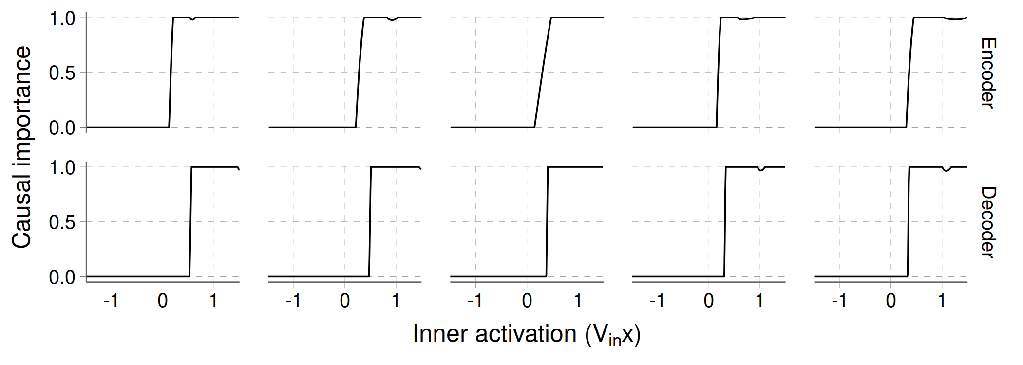
Notice how the activation thresholds tend to be a bit higher for the decoder, as they have to deal with interference between hidden features.
To push this further: since the process we use to predict causal importances is barred from taking an active role in reconstructing the output, it means we can make this process as sophisticated as we want – MLPs are fine for toy models, but something more expressive could be used if more complex models require it.
The clustering process is still in development. One way to go about it is to extend the "minimal description length" paradigm, so that multiple subcomponents can be grouped as one entity.
The causal-importance MLPs used during decomposition can already give you an estimate of which components are active or not, but you can probably come up with something fancier and more accurate.