Is there a reason you did 300/400 randomly sampled indices, instead of evenly spaced indices (e.g. every 1/300 of the total training steps)?
Did you subtract the mean of the weights before doing the SVD? Otherwise, the first component is probably the mean of the 300/400 weight vectors.
Btw, Neel Nanda has done similar experiments to your SVD experiment on his grokking models. For example, if we sample 400 datapoints from his mainline model, and cocatenate them into a [400, 226825] matrix, it turns out that the singular values are even more extreme than in your case: (apologies for the sloppily made figure)
(By your 10% threshold, it turns out only 5 singular values!)
We're pretty sure that component 0 is the "memorization" component, as it is dense in the Fourier basis while the other 4 big components are sparse, and then subtracting it from the model leads to better generalization.
Unfortunately, interpreting the other big ones turned out to be pretty non-trivial. This is despite the fact that many parts of the final network have low-rank approximations that capture >99% of the variance, we know the network is getting more sparse in the Fourier basis, and the entire function of the network is well known enough that you can literally read off the trig identities being used at the MLP layer. So I'm not super confident that purely unsupervised linear methods actually will help much with interpretability here.
(Also, having worked with this particular environment,I've seen a lot of further evidence that techniques like SVD and PCA are pretty bad for finding interpretable components.)
Another interesting experiment you might want to do is to look at the principal components of loss over the course of training, as they do in the Anthropic Induction Heads paper. 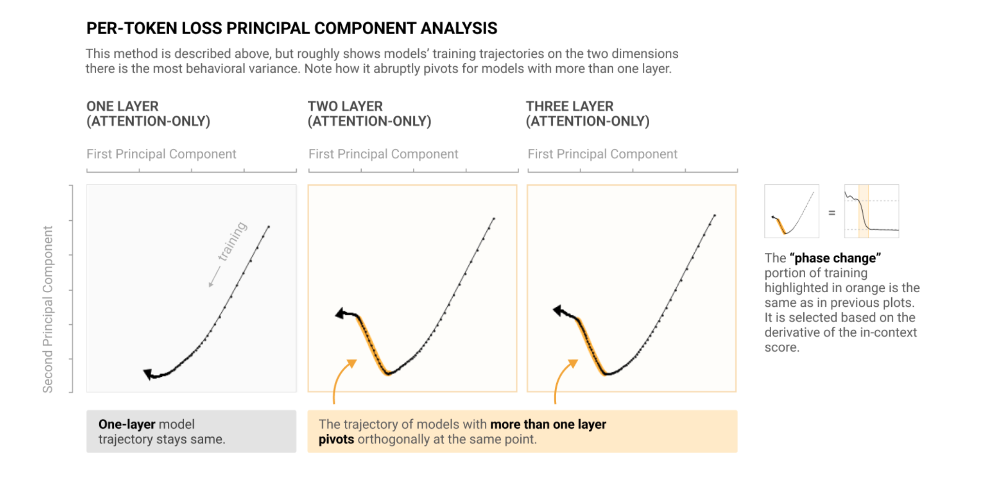
You can also plot the first two principal components of the logits, which in Neel's case gives a pretty diagram that shows two inflection points at checkpoints 14 and 103, corresponding to the change between the memorization phase (Checkpoint 0->14, steps 0->1.4k) and the circuit formation phase (Checkpoint 14 ->103, steps 1.4k -> 10.3k), and between the circuit formation phase and the cleanup phase (103->400, 10.3k->40k), which marks the start of grokking. Again, I'm not sure how illuminating figures like this actually are; it basically just says "something interesting happens around ~1.4k and ~10.3k, which we know from inspection of any of the other metrics (e.g. train/test loss). 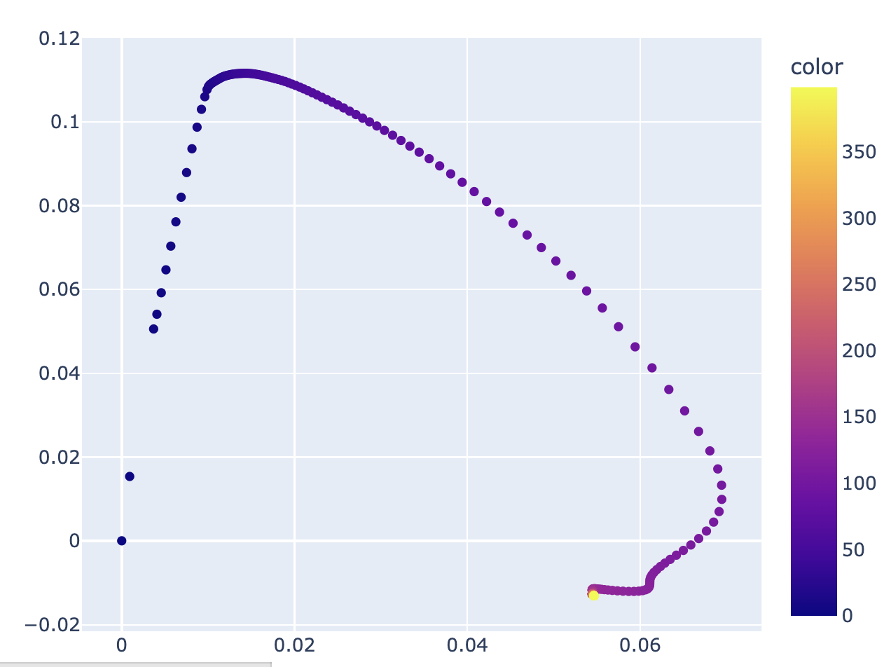
(In this case, there's a very good reason why looking the top 2 principal components of the logits isn't super illuminating: there's 1 "memorizing" direction and 5 "generalizing" directions, corresponding to each of the 5 key frequencies, on top of the normal interpretability problems.)
The main thing I want to do now is replicate the results from a particular paper whose name I can't remember right now, where an RL agent was trained to navigate to a cheese in the top right corner of a maze, apply this method to the training gradients, and see whether we can locate which parameters are responsible for the
if bottom_left(), then navigate_to_top_right()cognition, and which are responsible for theif top_right(), then navigate_to_cheese()cognition, which should be determinable by their time-step distribution.
Probably the easiest environment to run this on are the examples from Lauro Langosco's Goal Misgeneralization paper.
Another thought:
The main thing I want to do now is replicate the results from a particular paper whose name I can't remember right now, where an RL agent was trained to navigate to a cheese in the top right corner of a maze, apply this method to the training gradients, and see whether we can locate which parameters are responsible for the
if bottom_left(), then navigate_to_top_right()cognition, and which are responsible for theif top_right(), then navigate_to_cheese()cognition, which should be determinable by their time-step distribution.That is,
if bottom_left(), then navigate_to_top_right()should be associated with reinforcement events sooner during training rather than later, so the left singular values locating parameters responsible for that computation should have corresponding right singular values with high-in-magnitude numbers in their beginnings and low-in-magnitude numbers in their ends. Similarly,if top_right(), then navigate_to_cheese()should be associated with reinforcement events later during training, so the opposite holds.Then I want to verify that we have indeed found the right parameters by ablating the model's tendency to go to the cheese after its reached the top right corner.
It would also be interesting to see whether we can ablate the ability for it to go to the top right corner while keeping the ability to go to the cheese if the cheese is sufficiently close or it is already in the top right corner. However this seems harder, and not as clearly possible given we've found the correct parameters.
I might be missing something, but is there a reason you're doing this via SVD on gradients, instead of SVD on weights?
Is there a reason to do this with SVD at all, instead of mechanistic interp methods like causal scrubbing/causal tracing/path patching or manual inspection of circuits?
Is there a reason you did 300/400 randomly sampled indices, instead of evenly spaced indices (e.g. every 1/300 of the total training steps)?
No!
Did you subtract the mean of the weights before doing the SVD? Otherwise, the first component is probably the mean of the 300/400 weight vectors.
Ah, this is a good idea! I'll make sure to incorporate it, thanks!
Unfortunately, interpreting the other big ones turned out to be pretty non-trivial. This is despite the fact that many parts of the final network have low-rank approximations that capture >99% of the variance, we know the network is getting more sparse in the Fourier basis, and the entire function of the network is well known enough that you can literally read off the trig identities being used at the MLP layer. So I'm not super confident that purely unsupervised linear methods actually will help much with interpretability here.
Interesting. I'll be sure to read what he's written to see if its what I'd do.
Probably the easiest environment to run this on are the examples from Lauro Langosco's Goal Misgeneralization paper.
Thanks for the pointer, and thanks for the overall very helpful comment!
Thoughts, mostly on an alternative set of next experiments:
I find interpolations of effects to be a more intuitive way to study treatment effects, especially if I can modulate the treatment down to zero in a way that smoothly and predictably approaches the null case. It's not exactly clear to me what the "nothing going on case is", but here's some possible experiments to interpolate between it and your treatment case.
- alpha interpolation noise: A * noise + (A - 1) * MNIST, where the null case is the all-noise case. Worth probably trying out a bunch of different noise models since mnist doesn't really look at all gaussian.
- shuffle noise: Also worth looking at pixel/row/column shuffles, within an example or across dataset, as a way of preserving some per-pixel statistics while still reducing the structure of the dataset to basically noise. Here the null case is again that "fully noised" data should be the "nothing interesting" case, but we don't have to do work to keep per-pixel-statistics constant
- data class interpolation: I think the simplest version of this is dropping numbers, and maybe just looking at structurally similar numbers (e.g. 1,7 vs 1,7,9). This doesn't smoothly interpolate, but still having a ton of different comparisons with different subsets of the numbers. The null case here is that more digits adds more structure
- data size interpolation: downscaling the images, with or without noise, should reduce the structure such that the small / less data an example has, the closer it resembles the null case
- suboptimal initializations: neural networks are pretty hard to train (and can often degenerate) if initialized incorrectly. I think as you move away from optimal initialization (both of model parameters and optimizer parameters), it should approach the null / nothing interesting case.
- model dimensionality reduction: similar to intrinsic dimensionality, you can artificially reduce the (linear) degrees of freedom of the model without significant decrease to its expressivity by projecting into a smaller subspace. I think you'd need to get clever about this, because i think the naive version would just be linear projection before your linear operation (and then basically a no-op).
I mostly say all this because I think it's hard to evaluate "something is up" (predictions dont match empirical results) in ML that look like single experiments or A-B tests. It's too easy (IMO) to get bugs/etc. Smoothly interpolating effects, with one side as a well established null case / prior case, and another different case; which vary smoothly with whatever treatment, is IMO strong evidence that "something is up".
Hope there's something in those that's interesting and/or useful. If you haven't already, I strongly recommend checking out the intrinsic dimensionality paper -- you might get some mileage by swapping your cutoff point for their phase change measurement point.
So, just to check I understand:
At any given point in the optimization process, we have a model mapping input image to (in this case) digit classification. We also have a big pile of test data and ground-truth classifications, so we can compute some measure of how close the model is to confidently classifying every test case correctly. And we can calculate the gradient of that w.r.t. the model's parameters, indicating (1) what direction you want to make a small update in to improve the model and (2) what direction we actually do make a small update in at the next stage in the training process.
And you've taken all those gradient vectors and found, roughly speaking, that they come close to all lying in a somewhat lower-dimensional space than that of "all possible gradient vectors".
Some ignorant questions. (I am far from being an SVD expert.)
- As the optimization process proceeds, the updates will get smaller. Is it possible that (roughly speaking) the low-dimensional space you're seeing is "just" the space of update vectors from early in the process? (Toy example: suppose we have a 1000-dimensional space and the nth update is in the direction of the nth basis vector and has magnitude 1/n, and we do 1000 update steps. Then the matrix we're SVDing is diagonal, the SVD will look like identity . diagonal . identity, and the graph of singular values will look not entirely unlike the graphs you've shown.)
- Have you tried doing similar things with other highish-dimensional optimization processes, and seeing whether they produce similar results or different ones? (If they produce similar results, then probably what you're seeing is a consequence of some general property of such optimization processes. If they produce very different results, then it's more likely that what you're seeing is specific to the specific process you're looking at.)
- As the optimization process proceeds, the updates will get smaller. Is it possible that (roughly speaking) the low-dimensional space you're seeing is "just" the space of update vectors from early in the process? (Toy example: suppose we have a 1000-dimensional space and the nth update is in the direction of the nth basis vector and has magnitude 1/n, and we do 1000 update steps. Then the matrix we're SVDing is diagonal, the SVD will look like identity . diagonal . identity, and the graph of singular values will look not entirely unlike the graphs you've shown.)
It's definitely the case that including earlier updates leads to different singular vectors than if you exclude them. But it's not clear whether you should care about the earlier updates vs the later ones!
Oh yeah, I just remembered I had a way to figure out whether we’re actually getting a good approximation from our cutoff: look at what happens if you use the induced low rank approximation gradient update matrix as your gradients, then look at the loss of your alt model.
- This is a good hypothesis, and seems like it can be checked by removing the first however many timesteps from the svd calculation
- I have! I tried the same thing on a simpler network trained on an algorithmic task, and got similar results. In that case I got 10 singular vectors on 8M(?) time steps.
I googled around for what you'd expect from the SVD of random matrices, turns out to be a thing. Probably a better null hypothesis.
(work in progress) Colab notebook here.
Summary
I perform a singular value decomposition on a time series matrix of gradient updates from the training of a basic MNIST network across 2 epochs (≈2,000 time-steps), and find 92.5±11.6 singular values, about 4.625%±0.58% of what would be expected if there was nothing interesting going on. Then I propose various possible interpretations of the results including the left singular vectors representing capability phase changes, their representing some dependency structure across cognition, and their representing some indication of what could be considered a shard. Then I outline a particular track of experimentation I'd like to do to get a better understanding of what's going on here, and ask interested capable programmers, people with >0 hours of RL experience, or people with a decent amount of linear algebra experience for help or a collaborative partnership by setting up a meeting with me.
What is SVD
Very intuitive, low technical detail explanation
Imagine you have some physical system you'd like to study, and this physical system can be described accurately by some linear transformation you've figured out. What the singular value decomposition does is tell you the correct frame in which to view the physical system's inputs and outputs, so that the value of each of your reframed outputs is completely determined by the value of only one of your reframed inputs. The SVD gives you a very straightforward representation of naively quite messy situation.
Less intuitive, medium technical detail
All matrices can be described as a high dimensional rotation, various stretches along different directions, then another high dimensional rotation. The high dimensional rotations correspond to the frame shifts in the previous explanation, and the stretches correspond to the 'the value of each of your reframed outputs is completely determined by the value of only one of your reframed inputs' property.
Not intuitive, lots of technical detail
From Wikipedia
What did I do?
At each gradient step (batch) I saved the gradient of the loss with respect to the parameters of the model, flattened these gradients, and stacked them on top of each other to get a number-of-parameters×1 size vector, then I put all these vectors into a big matrix, so that the ith row represtented the ith parameter, and the jth column represented the jth gradient step.
Doing this for 2 epochs on a basic MNIST network gave me a giant number-of-parameters×≈2,000 size matrix.
I tried doing an SVD to this, but this crashed my computer, so instead I randomly sampled time-steps with which to do an SVD to (deleting the time steps not randomly sampled), and verified that the residual of the singular vectors with respect to a bunch of the other time step gradients was low. I found that if you randomly sampled about 300 time steps, this gives you a pretty low residual (≈1).
What we'd expect if nothing went on
If nothing interesting was going on we would expect about 2,000 nonzero singular values (since number-of-parameters>2,000), or at least some large fraction of 2,000 nonzero singular values.
If some stuff was going on, we would expect a lowish fraction (like 20-60%) of 2,000 nonzero singular values. This would be an interesting result, but not particularly useful, since 20-60% of 2,000 is still a lot, and this probably means lots of what we care about isn't being captured by the SVD reframing.
If very interesting stuff was going on, we would expect some very small fraction of 2,000 singular values. Like, <10%.
What we actually see
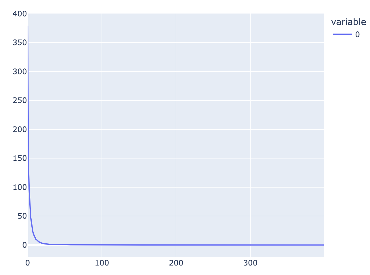
This is the graph of normalized singular values I found
And here's what we have for 400 randomly sampled indices just so you know it doesn't really change if you add more.
The x-axis is the singular value's index, and the y axis is the singular value's... well... value.
The rule of thumb is that all singular values less than 10% of the largest singular value are irrelevant, so what this graph tells us is that we have like 70-150 singular values[1], about 3.5-7.5% of what we would expect if nothing interesting was going on.
I ran this procedure (minus the graphs) 10 times, with 400 samples each, and took an average of the number of singular values relatively greater than 0.1 I got, resulting in an average of 92.5 singular values, with a standard deviation of 11.6. In terms of percentages of the full dimension, this is 4.625%±0.58%.
Theories about what's going on
The following theories are not necessarily mutually exclusive.
Experiments here I'd like to run
The main thing I want to do now is replicate the results from a particular paper whose name I can't remember right now, where an RL agent was trained to navigate to a cheese in the top right corner of a maze, apply this method to the training gradients, and see whether we can locate which parameters are responsible for the
if bottom_left(), then navigate_to_top_right()cognition, and which are responsible for theif top_right(), then navigate_to_cheese()cognition, which should be determinable by their time-step distribution.[EDIT: The name of the paper turned out to be Goal Misgeneralization by Langosco et al., and I was slightly wrong about what it concluded. It found that the RL agent learned to go to the top right corner, and also if there was a cheese near it, go to that cheese. Slightly different from what I had remembered, but the experiments described seem simple to caste to this new situation.]
That is,
if bottom_left(), then navigate_to_top_right()should be associated with reinforcement events sooner during training rather than later, so the left singular values locating parameters responsible for that computation should have corresponding right singular values with high-in-magnitude numbers in their beginnings and low-in-magnitude numbers in their ends. Similarly,if top_right(), then navigate_to_cheese()should be associated with reinforcement events later during training, so the opposite holds.Then I want to verify that we have indeed found the right parameters by ablating the model's tendency to go to the cheese after its reached the top right corner.
It would also be interesting to see whether we can ablate the ability for it to go to the top right corner while keeping the ability to go to the cheese if the cheese is sufficiently close or it is already in the top right corner. However this seems harder, and not as clearly possible given we've found the correct parameters.
I'd then want to make the environment richer in a whole bunch of ways-I-have-not-yet-determined, like adding more subgoals like also finding stars. If we make it find stars and cheeses, can we ablate the ability for it to find stars? Perhaps we can't because it thinks of stars and cheese as being basically the same thing, so can't distinguish between the two. In that case, what do we have to do to the training dynamics to make sure we are able to ablate the ability for it to find stars but still find cheese?
Call for people to help
I am slow at programming and inexperienced at RL. If you are fast at programming, have >0 hr of experience at RL, or are good with linear algebra[2], and want to help do some very interesting alignment research, schedule a meeting with me! We can talk, and see if we're a good fit to work together on this. (you can also just comment underneath this post with your ideas!)
This is such a wide range because the graph is fairly flat in the 0.1 area. If I instead had decided on the cutoff being 0.15, then I would have gotten like 40 singular values, and if I'd decided on it being 0.05, I would have gotten 200.
You can never have too much linear algebra!