Let's test on my favorite example: most people in port city in glasses are not librarian but sailors.
Share of librarians in town multiplied by share of librarians who wear glasses = share of people in glasses in town multiplied by share of people in glasses who are librarians
Below is Opus 4.5 text where I asked it explain your post with librarians example:
Here's the translation:
Step 1: Multiplication rule for joint events
P(L and G)=P(L)⋅P(G∣L)P(L \text{ and } G) = P(L) \cdot P(G|L)P(L and G)=P(L)⋅P(G∣L)
This is the probability of meeting a person who is both a librarian and wears glasses. We take the proportion of librarians in the city and multiply by the proportion of them who wear glasses.
P(G and L)=P(G)⋅P(L∣G)P(G \text{ and } L) = P(G) \cdot P(L|G)P(G and L)=P(G)⋅P(L∣G)
The same event, but "from the other side": we take the proportion of all people wearing glasses and multiply by the proportion of librarians among them.
Step 2: This is the same event, therefore
P(L)⋅P(G∣L)=P(G)⋅P(L∣G)P(L) \cdot P(G|L) = P(G) \cdot P(L|G)P(L)⋅P(G∣L)=P(G)⋅P(L∣G)
Step 3: Divide by P(G)
P(L∣G)=P(G∣L)⋅P(L)P(G)P(L|G) = \frac{P(G|L) \cdot P(L)}{P(G)}P(L∣G)=P(G)P(G∣L)⋅P(L)
Substituting our numbers:
P(L∣G)=0.50⋅0.001P(G)P(L|G) = \frac{0.50 \cdot 0.001}{P(G)}P(L∣G)=P(G)0.50⋅0.001
Where P(G)P(G)P(G) is the overall proportion of people wearing glasses in the city (summed across all population groups).
This is why even a high probability P(G∣L)=0.50P(G|L) = 0.50P(G∣L)=0.50 doesn't help: it gets multiplied by the tiny P(L)=0.001P(L) = 0.001P(L)=0.001, and as a result P(L∣G)P(L|G)P(L∣G) ends up being small.
I think the example has more to do with applying the theorem, while the post is about deriving it, so I’m not sure the post helps with the example directly.
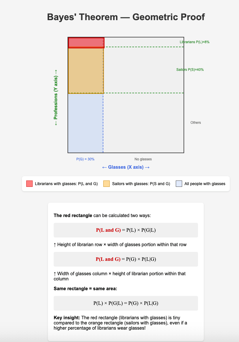
The example can be used to geometrically illustrate (and prove) the theorem. The whole city population can be represented as a square. On X axis is represented the number of people in the city in glasses. On Y axis, the number of people in with different professions. Below is AI generated image based on my prompt:
Your proof of Bayes' Theorem assumes P(A and B)=P(A)⋅P(B∣A), but it's not clear why someone who doubts Bayes would accept that.
That seems philosophically deeper than the goal of this post, which is to just help people who already accept the standard joint probability statement to remember Bayes’ Theorem. If I want to remember or write Bayes’ Theorem, I roughly just think “joint probability, divide.”
The intuition behind the definition there (it's a definition of conditional probability; the only assumption is that this correctly captures the informal idea of conditional probability) is: P(B) tells you how many worlds/how much probability mass is in the blob where B is true, measured so that if the blob contains everything then it has size 1. P(A|B) means you take the weight of A but constrain yourself to only look at worlds where B is true; so you look at the part of A that intersects B and measure it relative to B so that if it had B's size it would be 1. This is why you take P(A&B)/P(B).
Here's a table representing what's going on:
A -A
B w x
-B y z
where w = A & B, x = -A & B, etc.
Note that for example that probability of B = entire B row = w + x.
Now A|B means we keep only the B row and see what the chance of A is relative to it. This is why it's (A&B) / B - it's the upper left square over the upper row, because when we keep only the upper row we now need to compare squares to the new total of B. Likewise B|A means we keep only the A column and look at the relative change of B, so we get (A&B) / A
I find it easier to think in terms of odds, which are when you write only the relative probabilities (e.g. 1:2 odds and 2:4 odds both mean the same probabilities of 1/(1+2) = 1/3 vs 2/3). Here's a description of the intuition behind the proof, written in odds form:
Wordy description of odds form proof
The prior odds is the ratio of the A column to the -A column. The likelihood ratio is (B|A) : (B|-A), that is, each part is the "vertical factor" of the top row of a column compared to a whole column.
The first part of the likelihood ratio tells us how many B worlds each A world produces, while the second part tells us how many B worlds each -A world produces.
To get the total produced B worlds we multiply the prior (how many worlds we start out with) with the likelihood ratio (how many B worlds each one produces). Since we observed B, the posterior odds of A vs -A is the ratio between the "sources" of the B worlds, and so the product is our final odds.
Formally, we have
A : -A * (B | A) : (B | -A) = (A & B) : (-A & B)
and likewise
(A & B) : (-A & B) = B : B * (A | B) : (-A | B)
but since B : B = 1 : 1, this is just the desired (A | B) : (-A | B).
Example: Suppose that for every person with cancer there are 100 people with it. Then our prior odds are 1:100. If you get a cancer screening that will detect cancer 100% of the time if it's actually there but has a 10% of detecting it when it's not there, then the likelihood ratio is 100:10 = 10:1. The posterior odds of having cancer after you get a positive test result is then 1:100 * 10:1 = 1:10, which equivalently means you have a 1/11 posterior probability of having cancer.
I'm glad I know this, and maybe some people here don't, so here goes. P(A and B)=P(A)⋅P(B∣A) P(B and A)=P(B)⋅P(A∣B) Order doesn't matter for joint events: "A and B" refers to the same event as "B and A". Set them equal: P(B)⋅P(A∣B)=P(A)⋅P(B∣A) Divide by P(B): P(A∣B)=P(B∣A)⋅P(A)P(B) And you're done! I like substituting hypothesis (H) and evidence (E) to remember how this relates to real life: P(H∣E)=P(E∣H)⋅P(H)P(E)
You might also want to expand the denominator using the law of total probability, since you're more likely to know how probable the evidence is given different hypotheses than in general: P(Hi∣E)=P(E∣Hi)⋅P(Hi)∑jP(E∣Hj)⋅P(Hj)