This is a special post for quick takes by jacob_drori. Only they can create top-level comments. Comments here also appear on the Quick Takes page and All Posts page.
LLMs linearly represent the accuracy of their next-token predictions
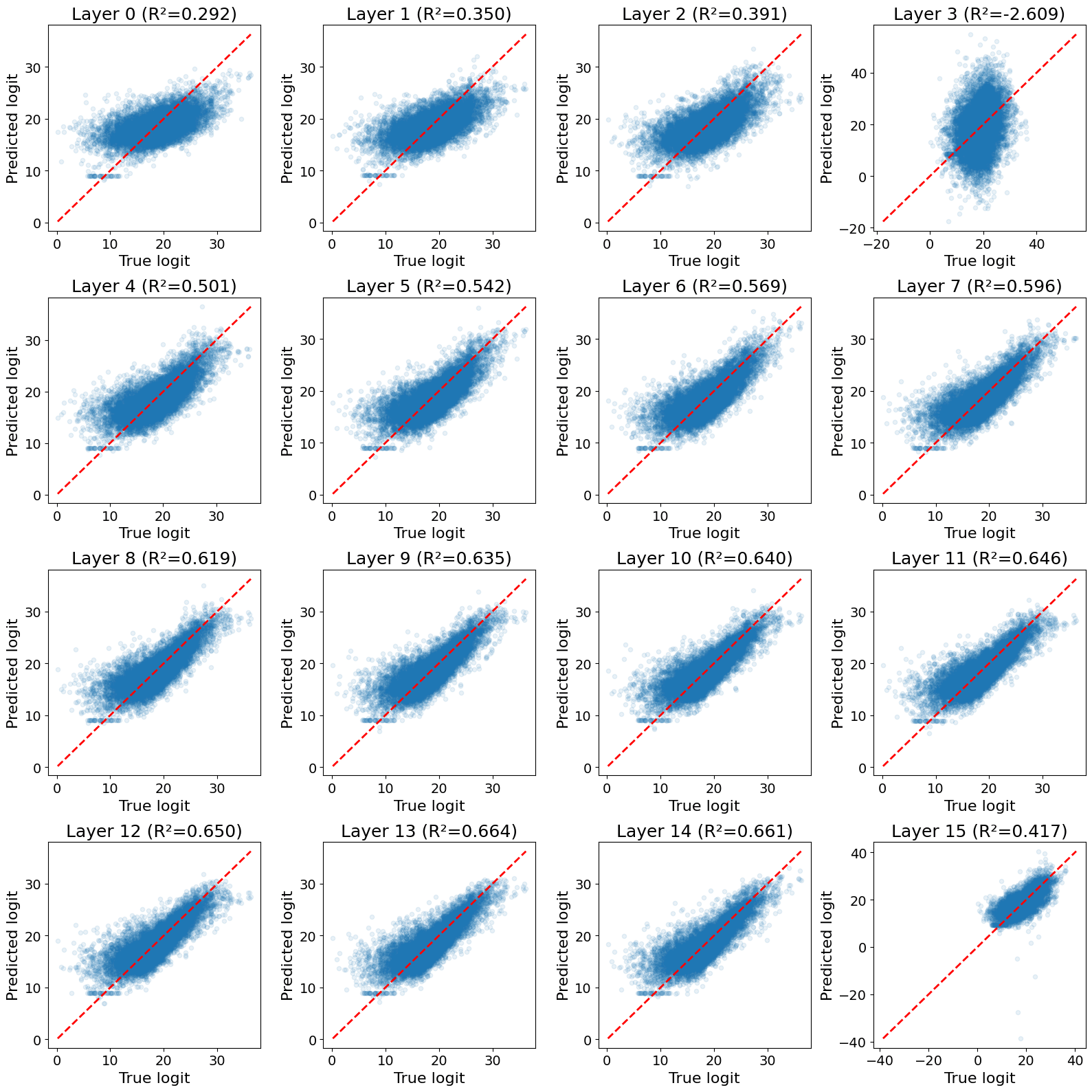
A quick experiment I did on Llama-3.2-1B:
- Choose a layer, and let be that layer's residual activation at token position .
- Let be the logit at position that was assigned to whatever turned out to be the correct next token (i.e. the correct token at position ).
- Use least-squares to fit a linear map that takes and predicts .
Results for each layer are below. Layers in the second half of the model (except the last layer) have decent () linear representations of the correct logit.
I don't find this result very surprising. I checked it because I thought it might explain what's going on in this very cool recent paper by @Dmitrii Krasheninnikov , Richard Turner and @David Scott Krueger (formerly: capybaralet)). They finetune Llama-3.2-1B and show that the model linearly represents the order of appearance of finetuning data. If more recent data has lower loss, then perhaps my probing results explain theirs.
Operationalizing the definition of a shard
Pope and Turner (2022) define a shard as follows:
A shard of value refers to the contextually activated computations which are downstream of similar historical reinforcement events.
To operationalize their definition, we must decide exactly what we mean by contextually activated computations, and by similar reinforcement events. One could philosophize here, but I'll just pick somewhat-arbitrary definitions and run with them, for the sake of quickly producing something I could turn into code.
Following Apollo/Goodfire, I will identify contextually activated computations with certain directions in parameter space. These directions might be found using APD, L3D, SPD, or some future method.
I am not sure when to consider two reinforcement events (i.e. RL reward-assignments) "similar". But if we replace "reinforcement events" with "RL updates", there is a natural definition: cluster RL parameter updates, and call two updates similar if they are in the same cluster. A given update should be allowed to be in multiple clusters, and we suspect parameter updates enjoy some linear structure. Therefore, a natural clustering method is an SAE.[1] Then, a shard is a decoder vector of an SAE trained on RL parameter updates.
Annoyingly, parameter vectors much larger than the activation vectors that SAEs are usually trained on, posing three potential issues:
- Storing enough parameter updates to train our SAE on takes a ton of memory.
- The SAE itself has a ton of parameters - too many to effectively train.
- It may be impossible to reconstruct parameter updates with reasonable sparsity (with , say, like standard SAEs).
To mitigate Issue 1, one could focus on a small subset of model parameters. One could also train the SAE at the same time as RL training itself, storing only a small buffer of the most recent parameter updates.
L3D cleverly deals with Issue 2 using low-rank parametrizations for the encoder and decoder of the SAE.
Issue 3 may turn out not to occur in practice. Mukherjee et al (2025) find that, when post-training an LLM with RL, parameter updates are very sparse in the neuron basis. Intuitively, many expect that such post-training merely boosts/suppresses a small number of pre-existing circuits. So perhaps we will find that, in practice, one can reconstruct parameter updates with reasonable sparsity.
All of this is to say: maybe someone should try training an SAE/applying L3D to RL parameter updates. And, if they feel like it, they could call the resulting feature vectors "shards".
Some issues with the ICL Superposition paper
Setup:
Xiong et al (2024) show that LLMs can in-context-learn several tasks at once. Consider e.g. the following prompt:
France -> F
Portugal -> Portuguese
Germany -> Berlin
Spain -> Madrid
Russia -> R
Poland -> Polish
Italy ->
A model will complete this prompt sometimes with Rome, sometimes with I, and sometimes with Italian, learning a "superposition" of the country -> capital, country -> first-letter and country -> language tasks. (I wish they hadn't used this word: the mech interp notion of superposition is unrelated).
Let be the proportion of the in-context examples that correspond to task , and let be the probability that the model completes the prompt according to task . Call a model calibrated if : the probability it assigns to a task is proportional to the number of times the task appeared in-context. A measure of the degree of calibration is given by the KL-divergence:
Lower KL means better calibration.
Issue 1:
The authors show that, for a certain set of 6 tasks, and with 60 in-context examples, calibration improves with model size:
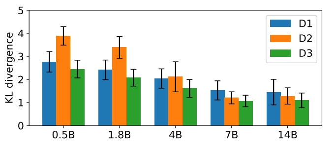
The best reported KL between the uniform distribution [0.167, 0.167, ..., 0.167] and the model's output distribution is around 1.5. To give a sense for what this means, here are four examples of distributions with such a KL:
.
Seeing these distributions convinced me that the models they studied are not well-calibrated. I felt a bit misled by the paper.
Issue 2:
Say we take turns with the model, repeatedly appending a new "question" (e.g. a country) to the prompt and allowing the model to generate an "answer" (e.g. the country's capital, language, or first letter) at default temperature 1.0. The authors state:
After the first token is generated, the model tends to converge on predicting tokens for a single task, effectively negating its ability for multi-task execution.
But this sort of mode-collapse behavior is not what we would observe from a well-calibrated model!
For simplicity, consider the case of only two tasks: and . Let and be the number of examples of each task, prior to a given generation step. A calibrated model generates with probability , in which case . Otherwise, it generates , and .
This is precisely the Pólya urn model. If the numbers of each task are initially and , and then we generate for a long time, it can be shown that the limiting proportion of tasks is a random variable distributed as follows:
In the realistic setting where , this distribution is peaked around, i.e. roughly the proportion of the initial tasks that were , and goes to zero at or . So calibrated models don't collapse; they tend to maintain roughly the initial ratio of tasks.