3 Answers sorted by
*
196I don't believe that the generating process for your simulation resembles that in the real world. If it doesn't, I don't see the value in such a simulation.
For an analysis of some situations where unmeasurably small correlations are associated with strong causal influences and high correlations (±0.99) are associated with the absence of direct causal links, see my paper "When causation does not imply correlation: robust violations of the Faithfulness axiom" (arXiv, in book). The situations where this happens are whenever control systems are present, and they are always present in biological and social systems.
Here are three further examples of how to get non-causal correlations and causal non-correlations. They all result from taking correlations between time series. People who work with time series data generally know about these pitfalls, but people who don't may not be aware of how easy it is to see mirages.
The first is the case of a bounded function and its integral. These have zero correlation with each other in any interval in which either of the two takes the same value at the beginning and the end. (The proof is simple and can be found in the paper of mine I cited.) For example, this is the relation between the current through a capacitor and the voltage across it. Set up a circuit in which you can turn a knob to change the voltage, and you will see the current vary according to how you twiddle the knob. Voltage is causing current. Set up a different circuit where a knob sets the current and you can use the current to cause the voltage. Over any interval in which the operating knob begins and ends in the same position, the correlation will be zero. People who deal with time series have techniques for detecting and removing integrations from the data.
The second is the correlation between two time series that both show a trend over time. This can produce arbitrarily high correlations between things that have nothing to do with each other, and therefore such a trend is not evidence of causation, even if you have a story to tell about how the two things are related. You always have to detrend the data first.
The third is the curious fact that if you take two independent paths of a Wiener process (one-dimensional Brownian motion), then no matter how frequently you sample them over however long a period of time, the distribution of the correlation coefficient remains very broad. Its expected value is zero, because the processes are independent and trend-free, but the autocorrelation of Brownian motion drastically reduces the effective sample size to about 5.5. Yes, even if you take a million samples from the two paths, it doesn't help. The paths themselves, never mind sampling from them, can have high correlation, easily as extreme as ±0.8. The phenomenon was noted in 1926, and a mathematical treatment given in "Yule's 'Nonsense Correlation' Solved!" (arXiv, journal). The figure of 5.5 comes from my own simulation of the process.
Thank for taking time to answer my question, as someone from the field!
The links you've given me are relevant to my question, and I can now rephrase my question as "in general, if we observe two things aren't correlated, how likely is it that one influences the other", or, simpler, how good is absence of correlation as evidence for absence of causation.
People tend to give examples of cases in which the absence of correlation goes hand in hand with the presence of causation, but I wasn't able to find an estimate of how often this occurs, which is potentiall...
163
The issue is trying to use an adjacency matrix as a causal influence matrix.
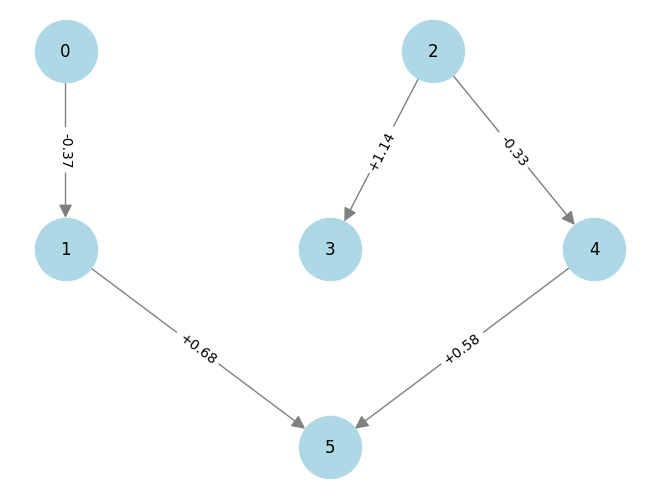
Let's say you have a graph with the following coefficients:
(0, 1): -0.371
(1, 5): +0.685
(2, 3): +1.139
(2, 4): -0.332
(4, 5): +0.580
which corresponds to a graph that looks like this
Working through the code step by step, with visualizations:
correlations = correlation_in_sem(sem, coefficients, inner_samples)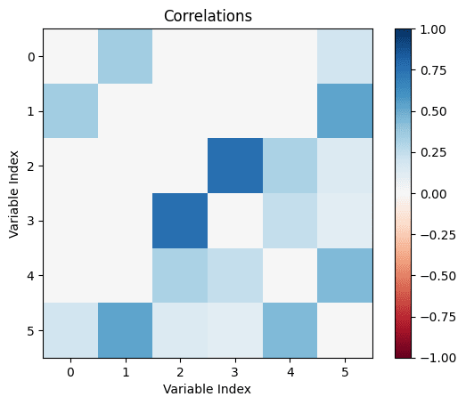
we see that, indeed, the correlations are what we expect (0 is uncorrelated with 2, 3, or 4 because there is no path from 0 to 2, 3, or 4 through the graph). Note that the diagonal is zeroed out.
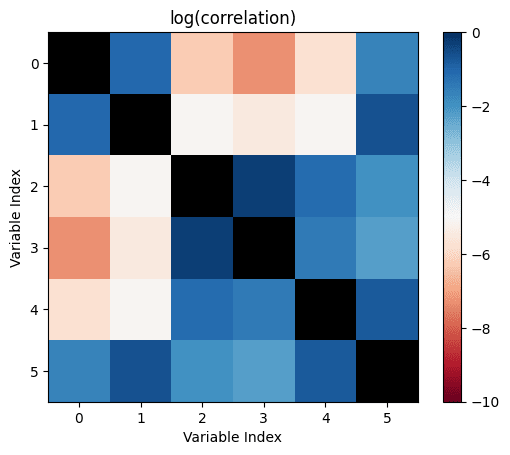
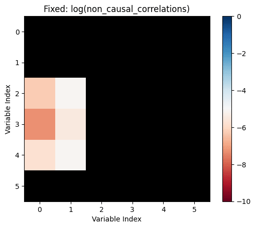
For the next step we are going to look at the log of the correlations, to demonstrate that they are nonzero even in the cases where there is no causal connection between variables:
We determine the adjacency matrix and then use that to determine the not_influence pairs, that is, the nodes where the first node does not affect the second
influence = nx.adjacency_matrix(sem).T.toarray().astype(bool)
not_influence = np.tril(~influence, -1)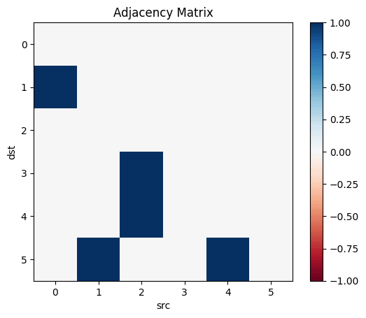
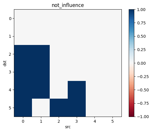
and

we see that, according to not_influence, node 0 has no effect on node 5.
So now we do
non_causal_correlations = not_influence * correlations
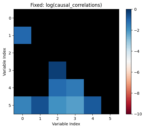
causal_correlations = influence * correlationsand see
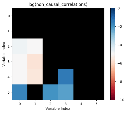
In order to fix this, we have to fix our influence matrix. A node src is causally linked to a node dst if the set of src and all its ancestors intersects with the set of dst and all its ancestors. In English "A is causally linked to B if A causes B, B causes A, or some common thing C causes both A and B".
influence_fixed = np.zeros((len(sem.nodes), len(sem.nodes)), dtype=bool)
for i in list(sem.nodes):
    for j in list(sem.nodes)[i+1:]:
        ancestry_i = nx.ancestors(sem, i).union({i})
        ancestry_j = nx.ancestors(sem, j).union({j})
        if len(ancestry_i.intersection(ancestry_j)) > 0:
            influence_fixed[j,i] = True
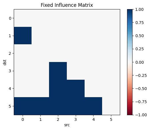
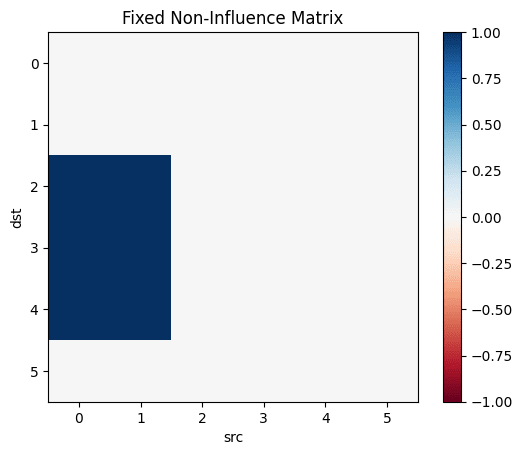
Looking again at the graph, this looks right.
- Node 0 directly affects node 1 and indirectly affects 5
- Node 1 directly affects node 5
- Node 2 directly affects 3 and 4 and indirectly affects 5
- Node 3 shares a common cause (2) with nodes 4 and 5
- Node 4 directly affects node 5
- Node 5 is the most-downstream node
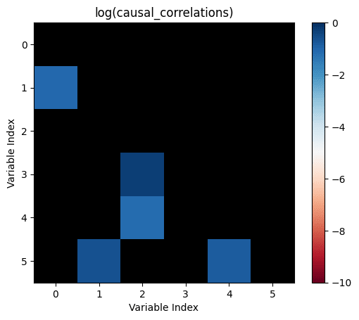
and now redrawing the correlations
Yes, thank you. Strong upvote. In a previous version I'd had I noticed this yesterday before going to sleep, let me fix the code and run it again (and update the post).
In a previous version I did use actual causal influence, not just direct nodes. The fixed code then is
influence=Matrix(Bool.(transpose(adjacency_matrix(transitiveclosure(sem)))))
instead of
influence=Matrix(Bool.(transpose(adjacency_matrix(sem))))
Interestingly, this makes the number of causal relationships higher, and should therefore also increase the number of causal non-correlations (which is also what now running the code suggests).
21
I think different people mean different things with "causation".
On the one hand, we have things where A makes B vastly more likely. No lawyer tries to argue that while their client shot the victim in the head (A) and the victim died (B), it could still be the case that the cause of death was old age and their client was simply unlucky. This is the strictest useful definition of causation.
Things get more complicated when A is just one of many factors contributing to B. Nine (or so) of ten lung carcinoma are "caused" by smoking, we say. But for the individual smoker cancer patient, we can only give a probability that their smoking was the cause.
On the far side, on priors I find it likely that the genes which determine eye colors in humans might also influence the chance that they get depression due to a long causal chain in the human body. Perhaps blue eyed people have an extra or chance to get depression compared to green eyed people after correcting for all the confounders, or perhaps it is the other way round. So some eye colors are possibly what one might call a risk factor for depression. This would be the loosest (debatably) useful definition of causation.
For such very weak "causations", a failure to find a significant correlation does not imply that there is no "causation". Instead, the best we can do is say something like "The likelihood of the observed evidence in any universe where eye color increases the depression risk by more than a factor of (or whatever) is less than one in 3.5 millions." That is, we provide bounds instead of just saying there is no correlation.
Current best guess: Nearly all the time55%.
"Correlation ⇏ Causation" is trite by now. And we also know that the contrapositive is false too: "¬Correlation ⇏ ¬Causation".
Spencer Greenberg summarizes:
I, however, have an inner computer scientist.
And he demands answers.
He will not rest until he knows how often ¬Correlation ⇒ ¬Causation, and how often it doesn't.
This can be tested by creating a Monte-Carlo simulation over random linear structural equation models with n variables, computing the correlations between the different variables for random inputs, and checking whether the correlations being zero implies that there is no causation.
So we start by generating a random linear SEM with n variables (code in Julia). The parameters are normally distributed with mean 0 and variance 1.
We can then run a bunch of inputs through that model, and compute their correlations:
We can then check how many correlations are "incorrectly small".
Let's take all the correlations between variables which don't have any causal relationship. The largest of those is the "largest uncaused correlation". Correlations between two variables which cause each other but are smaller than the largest uncaused correlation are "too small": There is a causation but it's not detected.
We return the amount of those:
And, in the outermost loop, we compute the number of misclassifications for a number of linear SEMs:
So we collect a bunch of samples. SEMs with one, two and three variables are ignored because when running the code, they never give me any causal non-correlations. (I'd be interested in seeing examples to the contrary.)
We can now first calculate the mean number of mistaken correlations and the proportion of misclassified correlations, using the formula for the triangular number:
So it looks like a growing proportion of causal relationships are not correlational, and I think the number will asymptote to include almost all causal relations55%.
It could also be that the proportion asymptotes to another percentage, but I don't think so15%.
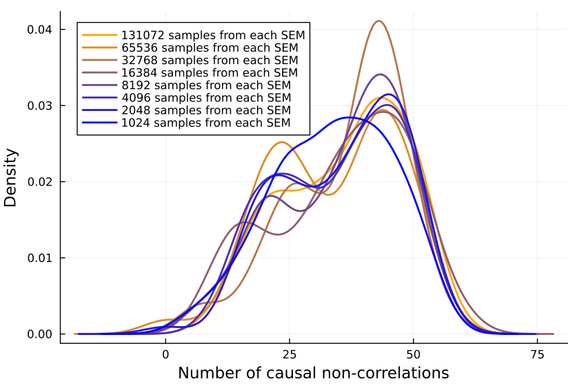
Is the Sample Size Too Small?
Is the issue with the number of inner samples, are we simply not checking enough? But 10k samples ought to be enough for anybody—if that's not sufficient, I don't know what is.
But let's better go and write some code to check:
Plotting the number of causal non-correlations reveals that 10k samples ought to be enough, at least for small numbers of variables:
The densities fluctuate, sure, but not so much that I'll throw out the baby with the bathwater. If I was a better person, I'd make a statistical test here, but alas, I am not.