Thanks for running these experiments and writing this up! I’m very excited to see this sort of followup work, and I think there are a lot of useful results here. I agree with most of this, and mostly just have a few nitpicks about how you interpret some things.
Reactions to the summary of your experimental results:
- CCS does so better than random, but not by a huge margin: on average, random linear probes have a 75% accuracy on some “easy” datasets;
- I think it’s cool that random directions sometimes do so well; this provides a bit of additional evidence that high-accuracy directions can be quite salient.
- It’s not too surprising to me that this holds for UQA (which is instruction-tuned, so it should intuitively have a particularly salient truth-y direction) and the easiest datasets like IMDB, but I doubt this holds for most models and datasets. At the very least I recall looking at this in one narrow setting before and got close to random performance (though I don’t remember what setting that was exactly). I’d be curious to see this for more model/dataset pairs.
- This is more of a nitpick with your phrasing, but FWIW based on the plot it does still look to me like CCS is better by a large margin (e.g. 75% accuracy to 95% accuracy is a 5x reduction in error) even in the settings where random directions do best. The takeaway for me here is mostly just that random direction can sometimes be surprisingly good -- which I agree is interesting.
- CCS does not find the single linear probe with high accuracy: there are more than 20 orthogonal linear probes (i.e. using completely different information) that have similar accuracies as the linear probe found by CCS (for most datasets);
- Yep, I agree; we definitely weren’t claiming to find a uniquely good direction. I also quite like the recursive CCS experiment, and would love to see more experiments along these lines.
- I think it’s interesting that you can find 20 orthogonal probes each with high accuracy. But I’m especially interested in how many functionally equivalent directions there are. For example, if this 20 dimensional subspace actually corresponds to roughly the same clustering into true and false, then I would say they are ~equivalent for my purposes.
- CCS does not always find a probe with low test CCS loss (Figure 1 of the paper is misleading). CSS finds probes which are sometimes overconfident in inconsistent predictions on the test set, resulting in a test loss that is sometimes higher than always predicting a constant probability;
- We indeed forgot to specify that figure 1 is with the train set — that was a good catch that we’ll specify in the arxiv version soon (we’ve already done so for the camera ready version).
- I think some of your experiments here are also interesting and helpful. That said, I do want to emphasize that I don’t find train-test distinctions particularly essential here because our method is unsupervised; I ultimately just want to find a direction that gives correct predictions to superhuman examples, and we can always provide those superhuman examples as part of the training data.
- Another way of putting this is that I view our method as being an unsupervised clustering method, for which I mostly just care about finding high-accuracy clusters. We also show it generalizes/transfers, but IMO that’s of secondary importance.
- I also think it's interesting to look at loss rather than just accuracy (which we didn't do much), but I do ultimately think accuracy is quite a bit more important overall.
- CCS’ performance on GPT-J heavily depends on the last tokens of the input, especially when looking at the last layers’ activations (the setting used in the paper).
- Thanks, these are helpful results. The experiment showing that intermediate layers can be better in some ways also feel similar to our finding that intermediate layers do better than later layers when using a misleading prompt. In general I would indeed like to see more work trying to figure out what’s going on with autoregressive models like GPT-J.
Reactions to your main takeaways:
- However, we still don’t know if this feature corresponds to the model’s “beliefs”.
- I agree. (I also still doubt current models have “beliefs” in any deep sense)
- Future work should compare their work against the random probe baseline. Comparing to a 50% random guessing baseline is misleading, as random probes have higher accuracy than that.
- I agree, this seems like a good point.
- CCS will likely miss important information about the model’s beliefs because there is more than one linear probe which achieves low loss and high CCS accuracy, i.e. there is more than one truth-like feature… There are many orthogonal linear probes which achieve low loss and high CCS accuracy, i.e. there are many truth-like features. Narrowing down which linear probe corresponds to the model’s beliefs might be hard.
- I think your experiments here are quite interesting, but I still don’t think they show that there are many functionally different truth-like features, which is what I mostly care about. This is also why I don’t think this provides much evidence that “Narrowing down which linear probe corresponds to the model’s beliefs might be hard.” (If you have two well-separated clusters in high dimensional space, I would expect there to be a large space of separating hyperplanes — this is my current best guess for what’s going on with your results.)
- There exists a direction which contains all linearly available information about truth, i.e. you can’t train a linear classifier to classify true from untrue texts after projecting the activations along this direction. CCS doesn’t find it. This means CCS is ill-suited for ablation-related experiments.
- I definitely agree that vanilla CCS is ill-suited for ablation-related experiments; I think even supervised linear probes are probably not what we want for ablation-related experiments, and CCS is clearly worse than logistic regression.
- I like this experiment. This suggests to me that there really is just functionally one truth-like feature/direction. I agree your results imply that vanilla CCS is not finding this direction geometrically, but your results make me more optimistic we can actually find this direction using CCS and maybe just a little bit more work. For example, I’d be curious to see what happens if you first get predictions from CCS, then use those predictions to get two clusters, then take the difference in means between those induced clusters. Do you get a better direction?
- More generally I'm still interested in whether this has meaningfully different predictions from what CCS finds or not.
- Future work should use more data or more regularization than the original paper did if it wants to find features which are actually truth-like.
- This seems like a useful finding!
- To get clean results, use CCS on UQA, and don’t get too close to GPT models. Investigating when and why CCS sometimes fails with GPT models could be a promising research direction.
- I basically agree, though I would suggest studying non-instruction tuned encoder or encoder-decoder models like T5 or (vanilla) DeBERTa as well, since instruction tuning might affect things.
- When using CCS on GPT models, don’t use CCS only on the last layer, as probes trained on activations earlier in the network are less sensitive to the format of the input.
- This also seems like an interesting finding, thanks!
I don’t find train-test distinctions particularly essential here because our method is unsupervised
If I recall correctly, most unsupervised learning papers do have a test set. Perhaps the fact that the train and test are different kind of shows why you need a test set in the first place.
Ablating along the difference of the means makes both CCS & Supervised learning fail, i.e. reduce their accuracy to random guessing. Therefore:
- The fact that Recursive CCS finds many good direction is not due to some “intrinsic redundancy” of the data. There exist a single direction which contains all linearly available information.
- The fact that Recursive CCS finds strictly more than one good direction means that CCS is not efficient at locating all information related to truth: it is not able to find a direction which contains as much information as the direction found by taking the difference of the means. Note: Logistic Regression seems to be about as leaky as CCS. See INLP which is like Recursive CCS, but with Logistic Regression.
I don't think that's a fair characterization of what you found. Suppose, for example, that you're given a vector in whose th component is , where is a random variable with high variance, and are i.i.d. with mean and tiny variance. There is a direction which contains all the information about contained in the vector, namely the average of the coordinates. Subtracting out the mean of the coordinates from each coordinate will remove all information about . But the data is plenty redundant; there are orthogonal directions each of which contain almost all of the available information about , so a probe trained to recover that learns to just copy one of the coordinates will be pretty efficient at recovering . If the have variance (i.e. are just constants always equal to ), then there are orthogonal directions each of which contain all information about , and a probe that copies one of them is perfectly efficient at extracting all information about .
If you can find multiple orthogonal linear probes that each get good performance at recovering some feature, then something like this must be happening.
"Redundancy" depends on your definition, and I agree that I didn't choose a generous one.
Here is an even simpler example than yours: positive points are all at (1...1) and negative points are all at (-1...-1). Then all canonical directions are good classifiers. This is "high correlation redundancy" with the definition you want to use. There is high correlation redundancy in our toy examples and in actual datasets.
What I wanted to argue against is the naive view that you might have which could be "there is no hope of finding a direction which encodes all information because of redundancy", which I would call "high ablation redundancy". It's not the case that there is high ablation redundancy in both our toy examples (in mine, all information is along (1...1)), and in actual datasets.
What you're calling ablation redundancy is a measure of nonlinearity of the feature being measured, not any form of redundancy, and the view you quote doesn't make sense as stated, as nonlinearity, rather than redundancy, would be necessary for its conclusion. If you're trying to recover some feature , and there's any vector and scalar such that for all data (regardless of whether there are multiple such , which would happen if the data is contained in a proper affine subspace), then there is a direction such that projection along it makes it impossible for a linear probe to get any information about the value of . That direction is , where is the covariance matrix of the data. This works because if , then the random variables and are uncorrelated (since ), and thus is uncorrelated with .
If the data is normally distributed, then we can make this stronger. If there's a vector and a function such that (for example, if you're using a linear probe to get a binary classifier, where it classifies things based on whether the value of a linear function is above some threshhold), then projecting along removes all information about . This is because uncorrelated linear features of a multivariate normal distribution are independent, so if , then is independent of , and thus also of . So the reason what you're calling high ablation redundancy is rare is that low ablation redundancy is a consequence of the existence of any linear probe that gets good performance and the data not being too wildly non-Gaussian.
Yep, high ablation redundancy can only exist when features are nonlinear. Linear features are obviously removable with a rank-1 ablation, and you get them by running CCS/Logistic Regression/whatever. But I don't care about linear features since it's not what I care about since it's not the shape the features have (Logistic Regression & CCS can't remove the linear information).
The point is, the reason why CCS fails to remove linearly available information is not because the data "is too hard". Rather, it's because the feature is non-linear in a regular way, which makes CCS and Logistic Regression suck at finding the direction which contains all linearly available data (which exists in the context of "truth", just as it is in the context of gender and all the datasets on which RLACE has been tried).
I'm not sure why you don't like calling this "redundancy". A meaning of redundant is "able to be omitted without loss of meaning or function" (Lexico). So ablation redundancy is the normal kind of redundancy, where you can remove sth without losing the meaning. Here it's not redundant, you can remove a single direction and lose all the (linear) "meaning".
I'm not sure why you don't like calling this "redundancy". A meaning of redundant is "able to be omitted without loss of meaning or function" (Lexico). So ablation redundancy is the normal kind of redundancy, where you can remove sth without losing the meaning. Here it's not redundant, you can remove a single direction and lose all the (linear) "meaning".
Suppose your datapoints are (where the coordinates and are independent from the standard normal distribution), and the feature you're trying to measure is . A rank-1 linear probe will retain some information about the feature. Say your linear probe finds the coordinate. This gives you information about ; your expected value for this feature is now , an improvement over its a priori expected value of . If you ablate along this direction, all you're left with is the coordinate, which tells you exactly as much about the feature as the coordinate does, so this rank-1 ablation causes no loss in performance. But information is still lost when you lose the coordinate, namely the contribution of from the feature. The thing that you can still find after ablating away the direction is not redundant with the the rank-1 linear probe in the direction you started with, but just contributes the same amount towards the feature you're measuring.
The point is, the reason why CCS fails to remove linearly available information is not because the data "is too hard". Rather, it's because the feature is non-linear in a regular way, which makes CCS and Logistic Regression suck at finding the direction which contains all linearly available data (which exists in the context of "truth", just as it is in the context of gender and all the datasets on which RLACE has been tried).
Disagree. The reason CCS doesn't remove information is neither of those, but instead just that that's not what it's trained to do. It doesn't fail, but rather never makes any attempt. If you're trying to train a function such that and , then will achieve optimal loss just like will.
- CCS does not find the single linear probe with high accuracy: there are more than 20 orthogonal linear probes (i.e. using completely different information) that have similar accuracies as the linear probe found by CCS (for most datasets);
So what about an ensamble of the top 20 linear probes? Is it substantially better than using just the best one alone? I would expect so given that they are orthogonal, so they are using ~uncorrelated information.
I think that a (linear) ensemble of linear probes (trained with Logistic Regression) should never be better than a single linear probe (otherwise the optimizer would have just found this combined linear probe instead). Therefore, I don't expect that ensembling 20 linear CCS probe will increase performance much (and especially not beyond the performance of supervised linear regression).
Feel free to run the experiment if you're interested about it!
Probes initialized like Collin does in the zip file: a random spherical initialization (take a random Gaussian, and normalize it).
The LessWrong Review runs every year to select the posts that have most stood the test of time. This post is not yet eligible for review, but will be at the end of 2024. The top fifty or so posts are featured prominently on the site throughout the year.
Hopefully, the review is better than karma at judging enduring value. If we have accurate prediction markets on the review results, maybe we can have better incentives on LessWrong today. Will this post make the top fifty?
Thanks a lot for this post, I found it very helpful.
There exists a single direction which contains all linearly available information Previous work has found that, in most datasets, linearly available information can be removed with a single rank-one ablation by ablating along the difference of the means of the two classes.
The specific thing that you measure may be more a fact about linear algebra rather than a fact about LLMs or CCS.
For example, let's construct data which definitely has two linearly independent dimension that are each predictive of whether a point is positive or negative. I'm assuming here that positive/negative exactly corresponds to true/false for convenience (i.e., that all the original statements happened to be true), but I don't think it should matter to the argument.
# Initialize the dataset
p = np.random.normal(size=size)
n = np.random.normal(size=size)

# In the first and second dimensions, they can take values -1, -.5, 0, .5, 1
# The distributions are idiosyncratic for each, but all are predictive of the truth
# label
standard = [-1, -.5, 0, .5, 1]
p[:,0] = np.random.choice(standard, size=(100,), replace=True, p=[0, .1, .2, .3, .4])
n[:,0] = np.random.choice(standard, size=(100,), replace=True, p=[.6, .2, .1, .1, .0])
p[:,1] = np.random.choice(standard, size=(100,), replace=True, p=[0, .05, .05, .1, .8])
n[:,1] = np.random.choice(standard, size=(100,), replace=True, p=[.3, .3, .3, .1, .0])
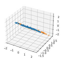
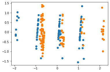
Then we can plot the data. For the unprojected data plotted in 3-d, the points are linearly classifiable with reasonable accuracy in both those dimensions.
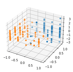
But then we perform the mean projection operation given here (in case I have any bugs!)
def project(p, n):
  # compute the means in each dim
  p_mean = np.mean(p, axis=0)
  n_mean = np.mean(n, axis=0)

  # find the direction
  delta = p_mean - n_mean
  norm = np.linalg.norm(delta, axis=0)
  unit_delta = delta / norm

  # project
  p_proj = p - np.expand_dims(np.inner(p, unit_delta),1) * unit_delta
  n_proj = n - np.expand_dims(np.inner(n, unit_delta),1) * unit_delta
  return p_proj, n_proj
And after projection there is no way to get a linear classifier that has decent accuracy.
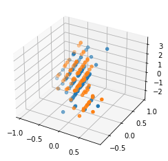
Or looking at the projection onto the 2-d plane to make things easier to see:
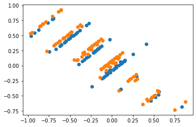
Note also that this is all with unnormalized raw data, doing the same thing with normalized data gives a very similar result with this as the unprojected:
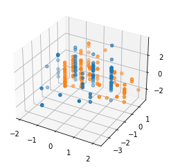
and these projected figures:
FWIW, I'm like 80% sure that Alex Mennen's comment gives mathematical intuition behind these visualizations, but it wasn't totally clear to me, so posting these in case it is clearer to some others as well.
I agree, there's nothing specific to neural network activations here. In particular, the visual intuition that if you translate the two datasets until they have the same mean (which is weaker than mean ablation), you will have a hard time finding a good linear classifier, doesn't rely on the shape of the data.
But it's not trivial or generally true either: the paper I linked to give some counterexamples of datasets where mean ablation doesn't prevent you from building a classifier with >50% accuracy. The rough idea is that the mean is weak to outliers, but outliers don't matter if you want to produce high-accuracy classifiers. Therefore, what you want is something like the median.
The fact that Recursive CCS finds strictly more than one good direction means that CCS is not efficient at locating all information related to truth: it is not able to find a direction which contains as much information as the direction found by taking the difference of the means. Note: Logistic Regression seems to be about as leaky as CCS.
Perhaps a naive question, but if a single linear projection exists that contains the desired information, why isn't this 'global minimum' found with LR (or CSS)?
That's because a classifier only needs to find a direction which correctly classifies the data, not a direction which makes other classifiers fail. A direction which removes all linearly available information is not always as good as the direction found with LR (at classification).
Maybe figure 2 from the paper which introduced mean difference as a way to remove linear information might help.
Thanks to Marius Hobbhahn and Oam Patel for helpful feedback on drafts. Thanks to Collin and Haotian for answering many questions about their work.
Discovering Latent Knowledge in Language Models Without Supervision describes Contrast-Consistent Search (CCS), a method to find a classifier which accurately answers yes-no questions given only unlabeled model activations. It might be a stepping stone towards recovering superhuman beliefs of AI systems, as unsupervised methods are more scalable and might be less likely to simply recover “what a human would say”.
I think this research direction is interesting and promising. But I feel like people often got a bit carried away with the approximate takeaway they got from the experimental results of the initial paper.
In this post, I present experimental results which highlight the strengths and weaknesses of CCS.
Main takeaways:
Experimental setup
I’m using a modified version[1] of the code Collin and Haotian used to run the experiments (the zip file linked in this readme).
I report results for two models:
For each model, I only use datasets which they can solve, i.e. datasets for which the accuracy of a linear probe trained with supervised labels on the last layer’s activation is at least 90%. All experiments are done with 10 random seeds.
What CCS does and doesn’t find
CCS is able to find a single probe which correctly classifies statements across datasets
What the paper does: It trains linear probes on individual datasets (IMDB, COPA, …), and then measures high transfer accuracies (Appendix E).
What Collin claims (in the Alignment Forum Post): “CCS, accurately classifies text as true or false directly from a model’s unlabeled activations across a wide range of tasks”. Right below, the figure only shows one theta instead of many thetas (one per task) may lead the reader to think that only one linear probe is trained across the wide range of tasks.
What I measure: I train a probe on all datasets (the “trained together” probe) each model can solve. I reproduce Collin’s experiments by training probes on each dataset. I evaluate accuracy on each dataset separately. I compare those two ways of finding probes with the “ceiling” used in the paper: training a supervised probe per dataset.
What I find: Training a single CCS probe does not reduce accuracy by a significant margin over training a probe per dataset, which supports the idea that CCS enables you to find a single probe which classifies text as true or false (a least for text inputs which are correctly answered questions from classic NLP datasets).
CCS does so better than random, but not by a huge margin
What the paper does: it never measures the accuracy of random probes
What Collin claims: “it wasn’t clear to me whether it should even be possible to classify examples as true or false from unlabeled LM representations better than random chance”
What I measure: I use the random initialization of CCS probes, but I don’t train them at all. Then I measure their accuracy.
Note: random accuracy can be better than 0.5 because the methodology used in the CCS paper allows you to swap all predictions if your accuracy is below 50%, and thereby extract one bit of information from the (test) labels. This is because the CCS loss isn’t able to distinguish the probes which correctly classify all statements from the probes which incorrectly classify all statements.
What I find: The accuracy of random linear probes is very high! But both CCS and supervised learning are above what you would expect if they were just getting random-but-lucky probes.
Implications: Future research should always compare their results with randomly initialized probes rather than with random guessing when it wants to assess how much CCS was able to single out a “good” probe. Other baselines such as zero-shot and Logistic Regression can be interesting but measure slightly different things.
The fact that even random probes can get relatively high accuracy hints towards the next point: there are many linear probes which get high accuracy.
CCS does not find the single linear probe with high accuracy
What the paper does: It does not try to measure if the probe CCS finds is unique.
What Collin claims: “Hypothesis 3: One of the few truth-like features GPT-n will represent is whether an input is actually true or false. This would mean that we only need a small number of remaining bits to identify its beliefs from all the candidate features”.
For the rest of this post, I will write about “directions” without specifying that I’m writing about the direction of a linear classifier i.e. the direction orthogonal to the decision plane of the classifier i.e the unit vector d in y = \sigma(a<d,x> + b). I will also use “direction” to speak about the feature it captures in the model’s activation.
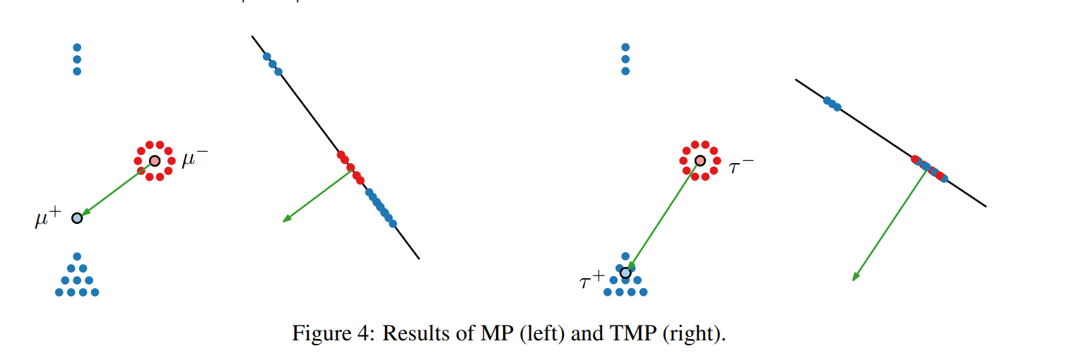
What I measure: I use CCS multiple times, constraining the direction of the linear classifier at iteration n to be orthogonal to the directions of the linear classifiers found by CCS at iteration 1, …, n-1 i.e. the nth probe can’t use information used by previous iterations. The original idea is from Nora Belrose, and I call this Recursive CCS (RCCS). I measure the accuracy of each probe found by the first 20 iterations of Recursive CCS.
What I find: Average accuracy decreases only slightly across the 20 iterations when training CCS probes on all datasets combined, especially on UnifiedQA (a model specifically trained for question answering). This means that there are at least 20 orthogonal directions which are good candidates for identifying the model “beliefs”. Vanilla CSS likely doesn’t find a unique truth-like direction but only one of many truth-like directions. This means that:
Note: Linear combinations of candidates are often good candidates themselves[2], so you need at least 20 bits of information to narrow down the right direction (20 is the number of bits needed to describe a linear combination when the weight of each orthogonal candidate is either 0 or 1). It’s not just the log2(20) bits you would need to distinguish between the 20 orthogonal directions found by Recursive CCS.
Iteration 1 is vanilla CCS, iteration 2 is CCS with the constraint that the direction should be orthogonal to the direction found by iteration 1, iterations 3 is CCS with the constraint that the direction should be orthogonal to the directions found by iterations 1 and 2, …
There are many good directions, does CCS always find roughly the same one?
What I measure: For a single dataset, I run CCS 10 times with different seeds, then measure cosine similarities between the directions of each seed: cosine_similarity(d[i], d[j]) for each i!=j.
What I find: CCS always find roughly the same direction, at least for directions of linear probes trained only on datasets where they have high accuracy (UQA, and GPT-J imdb). The cosine similarities between directions found by CCS across seeds is pretty big (in dimension 1024 (UQA) and 4096 (GPT-J), a cosine similarity of 0.4 is already quite big).
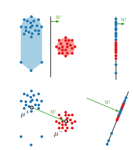
There exists a single direction which contains all linearly available information
Previous work has found that, in most datasets, linearly available information can be removed with a single rank-one ablation by ablating along the difference of the means of the two classes.
What I measure: I measure the difference of the means of normalized activations x of true and false statements: Δ=1|{i|y(i)=True}|∑i|y(i)=Truex(i)−1|{i|y(i)=False}|∑i|y(i)=Falsex(i). I then project the data along this direction: ^x=x−⟨x,Δ⟩Δ. Finally, I use CCS on ^x instead of x.
What I find: Ablating along the difference of the means makes both CCS & Supervised learning fail, i.e. reduce their accuracy to random guessing. Therefore:
As you can see below, after the ablation along the mean difference direction, accuracies are down to ~50%.
If instead, you ablate along the direction found by CCS, it gives you iteration 2 of Recursive CCS, which decreases accuracy by a tiny amount. For example, on UQA, for a probe trained on all datasets, ablating along the vanilla CCS direction makes the accuracy of CCS probes go from 92% to 91% (see the first figure of this section).
CCS does not find a probe with low test CCS loss
What the paper does: It does not report test loss. The only clue that might make us guess test loss is Figure 1, which shows the resulting probability distribution on the train set (it’s not stated in the text, but I’ve asked Collin about it).
What Collin claims: “[...] even if GPT-n represents its beliefs in its activations, our method might still find a different “truth-like” feature [...]”, which implies that CCS finds truth-like features.
What I measure: The most natural interpretation of a “truth-like” probe is a probe which has low CCS test loss. So I measure CCS loss on both probes trained on one dataset and on probes trained with dataset at once. I compare it with 0.2, the loss you would get by blindly predicting p=0.4 on every input, which minimizes the CCS loss[3]. I also reproduce Figure 1 on the train & test sets (with UQA and COPA, as the original paper did), because Figure 1 of the paper might make the reader believe that CCS finds a probe with low test loss.
What I find: Test loss is sometimes higher than the loss of 0.2 you would get with a constant prediction.
Left: figure of CCS results on training data, copied from paper; Right: replicated results applied to training and test set.
Interpretation: The probe is often very overconfident and has severely overfitted the training data. It often predicts that “Q? Yes” and “Q? No” are either both true or both untrue, resulting in the bump around 0.5. It is usually more confident in the right answer than overconfident in the wrong answer, and thus, the prediction is often correct even when one of p^+ or p^- is completely wrong, which is why CCS has still high test accuracy. The strength of CCS does not come from how truth-like the directions it has found are, it comes from finding some information about which parts of the activation space contain information relevant for predicting if the text is true or false (see diagram below).
Note: CCS is trained with some regularization (the default weight decay of 0.01 of AdamW). Removing regularization makes test loss much worse and somewhat decreases accuracy.
CCS’ performance on GPT-J depends heavily on the last tokens of the prompt
What the paper does: In all experiments of the paper, the last token is the answer (so that the prompt format is compatible with zero-shot predictions), even though it might matter a lot since CCS uses the activations of the model at the last position (i.e. the activations used to predict what comes right after the text).
What Collin claims: Collin claims that CCS “accurately classifies text as true or false”. He doesn’t specify constraints on the kind of text CCS is able to classify, and in particular never states that the end of the text should contain decisive information which makes the text true or false. He acknowledges that results on GPT-J are weak (“it seems like it might work less consistently in autoregressive models for reasons we don’t understand well”).
What I measure: I measure the impact of a distracting suffix at the end of the input, to see if CCS is able to find if statements are true or false even when last token isn’t the answer. The motivation for this is that if CCS actually measures truth-like features in a sentence, these features should be detectible at different positions of the sentence. Otherwise, the method is unlikely to generalize and find truth-like features in general text which is what we would ultimately want from CCS.
What I find:
Note: UQA’s encoder has 22 layers and GPT-J has 28 layers.
Interpretation (speculative):
Note: In the original paper, Appendix F shows accuracy across layers for every model. It shows that accuracy is very slightly better in GPT-J in the middle of the network. In the experiments I ran, where a suffix is present, the performance increase when looking earlier in the network is much bigger.
It’s still unclear to me why Logistic Regression performs well at the last layer of the network even when there is a distracting suffix.
What it implies for CCS: CCS can only work when information about the truth of a statement is clearly encoded in the network’s activations. This is not always the case at the last position of the last layer of an GPT models, which should only contain information relevant to predict the next token after the input text. Therefore, CCS should be used on activations of intermediate layers of the model instead of its last layer. This makes the method much more robust, and more likely to capture high level abstraction built by the model rather than correlations in the next token predicted by the model.
The original zip file and the original GitHub repo contain major bugs. If you want to work on CCS use either
- My repository, which has a relatively small diff with the original zip file,
- Or EleutherAI’s, which is still under development, supports GPU parallelism, has a structure very different from the original CCS code, and aims at extending CCS in radical ways.
If you change the magnitude and bias of the corresponding probe, the linear combination of two probes found by Recursive CCS has low loss and high accuracy. Experiments are not in this post (because I did them with an old codebase), but I might reproduce them and add them to the post if it matters to someone.
The loss is L = min(p0,p1)² + (p0 + p1 - 1)². If p0=p1=p (a blind constant guess), then L = p² + (2p² - 1)² which is minimum for p=0.4 for which L=0.2.