Crossposted from the AI Alignment Forum. May contain more technical jargon than usual.

Produced under the mentorship of Evan Hubinger as part of the SERI ML Alignment Theory Scholars Program - Winter 2022 Cohort

A big thank you to all of the people who gave me feedback on this post: Edmund Lao, Dan Murfet, Alexander Gietelink Oldenziel, Lucius Bushnaq, Rob Krzyzanowski, Alexandre Variengen, Jiri Hoogland, and Russell Goyder.

Statistical learning theory is lying to you: "overparametrized" models actually aren't overparametrized, and generalization is not just a question of broad basins.

The standard explanation thrown around here for why neural networks generalize well is that gradient descent settles in flat basins of the loss function. On the left, in a sharp minimum, the updates bounce the model around. Performance varies considerably with new examples. On the right, in a flat minimum, the updates settle to zero. Performance is stabler under perturbations.

To first order, that's because loss basins actually aren't basins but valleys, and at the base of these valleys lie "rivers" of constant, minimum loss. The higher the dimension of these minimum sets, the lower the effective dimensionality of your model.[1] Generalization is a balance between expressivity (more effective parameters) and simplicity (fewer effective parameters).

Symmetries lower the effective dimensionality of your model. In this example, a line of degenerate points effectively restricts the two-dimensional loss surface to one dimension.

In particular, it is the singularities of these minimum-loss sets — points at which the tangent is ill-defined — that determine generalization performance. The remarkable claim of singular learning theory (the subject of this post), is that "knowledge … to be discovered corresponds to singularities in general" [1]. Complex singularities make for simpler functions that generalize further.

The central claim of singular learning theory is that the singularities of the set of minima of the loss function determine learning behavior and generalization. Models close to more complex singularities generalize further.

Mechanistically, these minimum-loss sets result from the internal symmetries of NNs[2]: continuous variations of a given network's weights that implement the same calculation. Many of these symmetries are "generic" in that they are predetermined by the architecture and are always present. The more interesting symmetries are non-generic symmetries, which the model can form or break during training.

In terms of these non-generic symmetries, part of the power of NNs is that they can vary their effective dimensionality. Generality comes from a kind of internal model selection in which the model finds more complex singularities that use fewer effective parameters that favor simpler functions that generalize further.

At the risk of being elegance-sniped, SLT seems like a promising route to develop a better understanding of generalization and the limiting dynamics of training. If we're lucky, SLT may even enable us to construct a grand unified theory of scaling.

A lot still needs to be done (in terms of actual calculations, the theorists are still chewing on one-layer tanh models), but, from an initial survey, singular learning theory feels meatier than other explanations of generalization. It's more than just meatiness; there's a sense in which singular learning theory is a non-negotiable prerequisite for any theory of deep learning. Let's dig in.

Back to the Bayes-ics

Singular learning theory begins with four things:

  • The "truth", , which is some distribution that is generating our samples;
  • A model, parametrized by weights , where  is compact;
  • A prior over weights, ;
  • And a dataset of samples , where each random variable  is i.i.d. according to .

Here, I'm follow the original formulation and notation of Watanabe [1]. Note that most of this presentation transfers straightforwardly from the context of density estimation (modeling ) to other problems like regression and classification (modeling ) [2]. (I also am deeply indebted to Carroll's Msc. Thesis [2] and the wonderful seminars and notes at metauni [3])

The lower-level aim of "learning" is to find the optimal weights for the given dataset. As good Bayesians, this has a very specific and constrained meaning:

The higher-level aim of "learning" is to find the optimal model class/architecture, for the given dataset. Rather than try to find the weights that maximize the likelihood or even the posterior, the true aim of a Bayesian is to find the model that maximizes the model evidence,

The fact that the Bayesian paradigm can integrate out its weights to make statements over entire model classes is one of its main strengths. The fact that this integral is often almost always intractable is one of its main weaknesses. So the Bayesians make a concession to the frequentists with a much more tractable Laplace approximation: we find a choice of weights, , that maximizes the likelihood and then approximate the distribution as Gaussian in the vicinity of that point.

The Laplace Approximation is just a probability theorist's (second-order) Taylor expansion.

This is justified on the grounds that as the dataset grows (), thanks to the central limit theorem, the distribution becomes asymptotically normal (cf. physicists and their "every potential is a harmonic oscillator if you look closely enough / keep on lowering the temperature.").

From this approximation, a bit more math leads us to the following asymptotic form for the negative log evidence (in the limit ):

where  is the dimensionality of parameter space.

This formula is known as the Bayesian Information Criterion (BIC), and it (like the related Akaike information criterion) formalizes Occam's razor in the language of Bayesian statistics. We can end up with models that perform worse as long as they compensate by being simpler. (For the algorithmic-complexity-inclined, the BIC has an alternate interpretation as a device for minimizing the description length in an optimal coding context.)

Unfortunately, the BIC is wrong. Or at least the BIC doesn't apply for any of the models we actually care to study. Fortunately, singular learning theory can compute the correct asymptotic form and reveal its much broader implications.

Statistical learning theory is built on a lie

The key insight of Watanabe is that when the parameter-function map,

is not one-to-one, things get weird. That is, when different choices of weights implement the same functions, the tooling of conventional statistical learning theory breaks down. We call such models "non-identifiable".

When the parameter-function map is not one-to-one, the right object of study is not parameter space but function/distribution space.

Take the example of the Laplace approximation. If there's a local continuous symmetry in weight space, i.e., some direction you can walk that doesn't affect the probability density, then your density isn't locally Gaussian.

The Laplace approximation breaks down when there is a direction of perfect flatness.

Even if the symmetries are non-continuous, the model will not in general be asymptotically normal. In other words, the standard central limit theorem does not hold.

The same problem arises if you're looking at loss landscapes in standard presentations of machine learning. Here, you'll find attempts to measure basin volume by fitting a paraboloid to the Hessian of the loss landscape at the final trained weights. It's the same trick, and it runs into the same problem.

This isn't the kind of thing you can just solve by adding a small  to the Hessian and calling it a day. There are ways to recover "volumes", but they require care. So, as a practical takeaway, if you ever find yourself adding  to make your Hessians invertible, recognize that those zero directions are important to understanding what's really going on in the network. Offer those eigenvalues the respect they deserve.

Adding epsilon to fudge your paraboloids is a dirty, insidious practice.

The consequence of these zeros (and, yes, they really exist in NNs) is that they reduce the effective dimensionality of your model. A step in these directions doesn't change the actual model being implemented, so you have fewer parameters available to "do things" with.

So the basic problem is this: almost all of the models we actually care about (not just neural networks, but Bayesian networks, HMMs, mixture models, Boltzmann machines, etc.) are loaded with symmetries, and this means we can't apply the conventional tooling of statistical learning theory.

Learning is physics with likelihoods

Let's rewrite our beloved Bayes' update as follows,

where  is the negative log likelihood,

and ​ is the model evidence,

Notice that we've also snuck in an inverse "temperature", , so we're now in the tempered Bayes paradigm [4]. 

The immediate aim of this change is to emphasize the link with physics, where ​ is the preferred notation (and "partition function" the preferred name). The information theoretic analogue of the partition function is the free energy,

which will be the central object of our study.

Under the definition of a Hamiltonian (or "energy function"),

the connection is complete: statistical learning theory is just mathematical physics where the Hamiltonian is a random process given by the likelihood and prior. Just as the geometry of the energy landscape determines the behavior of the physical systems we study, the geometry of the log likelihood ends up determining the behavior of the learning systems we study.

In terms of this physical interpretation, the a posteriori distribution is the equilibrium state corresponding to this empirical Hamiltonian. The importance of the free energy is that it is the minimum of the free energy (not of the Hamiltonian) that determines the equilibrium.

Our next step will be to normalize these quantities of interest to make them easier to work with. For the negative log likelihood, this means subtracting its minimum value.[3] 

But that just gives us the KL divergence,

where ​ is the empirical entropy,

a term that is independent of .

The empirical Kullback-Leibler divergence is just a rescaled and shifted version of the negative log likelihood. Maximum likelihood estimation is equivalent to minimizing the empirical KL divergence.

Similarly, we normalize the partition function to get

and the free energy to get

This lets us rewrite the posterior as

The more important aim of this conversion is that now the minima of the term in the exponent, , are equal to 0. If we manage to find a way to express  as a polynomial, this lets us to pull in the powerful machinery of algebraic geometry, which studies the zeros of polynomials. We've turned our problem of probability theory and statistics into a problem of algebra and geometry.

Why "singular"?

Singular learning theory is "singular" because the "singularities" (where the tangent is ill-defined) of the set of your loss function's minima,

determine the asymptotic form of the free energy. Mathematically, ​ is an algebraic variety, which is just a manifold with optional singularities where it does not have to be locally Euclidean.

Example of the curve  (equivalently, the algebraic variety of the polynomial . [Source]

By default, it's difficult to study these varieties close to their singularities. In order to do so anyway, we need to "resolve the singularities." We construct another well-behaved geometric object whose "shadow" is the original object in a way that this new system keeps all the essential features of the original.

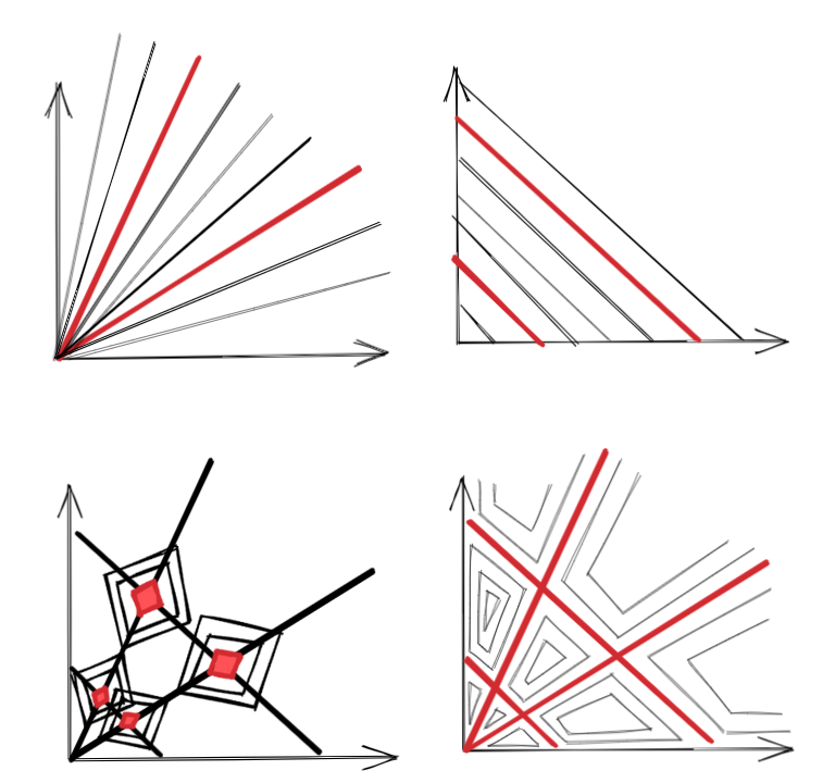
It'll help to take a look at the following figure. The main idea behind resolution of singularities is to create a new manifold  and a map , such that  is a polynomial in the local coordinates of . We "disentangle" the singularities so that in our new coordinates they cross "normally".

Based on Figure 2.5 of [1]. The lines represent the points that are in . The colors are just there to help you keep track of the points.

Because this "blow up" creates a new object, we have to be careful that the quantities we end up measuring don't change with the mapping — we want to find the birational invariants.

We are interested in one birational invariant in particular: the real log canonical threshold (RLCT). Roughly, this measures how "bad" a singularity is. More precisely, it measures the "effective dimensionality" near the singularity.

After fixing the central limit theorem to work in singular models, Watanabe goes on to derive the asymptotic form of the free energy as ,

where,   is the RLCT,  is the "multiplicity" associated to the RLCT,  is a (well-behaved) random variable, and  is a random variable that converges (in probability) to zero.

The important observation here is that the global behavior of your model is dominated by the local behavior of its "worst" singularities. 

For regular (=non-singular) models, the RLCT is , and with the right choice of inverse temperature, the formula above simplifies to

which is just the BIC, as expected.

The free energy formula generalizes the BIC from classical learning theory to singular learning theory, which strictly includes regular learning theory as a special case. We see that singularities act as a kind of implicit regularization that penalizes models with higher effective dimensionality.

Phase transitions are singularity manipulations

Minimizing the free energy is maximizing the model evidence, which, as we saw, is the preferred Bayesian way of doing model selection. Other paradigms may disagree[4], but at least among us this makes minimizing the free energy the central aim of statistical learning.

As in statistical learning, so in physics.

In physical systems, we distinguish microstates, such as the particular position and speed of every particle in a gas, with macrostates, such as the values of the volume and pressure. The fact that the mapping from microstates to macrostates is not one-to-one is the starting point for statistical physics: uniform distributions over microstates lead to much more interesting distributions over macrostates.

Often, we're interested in how continuously varying our levers (like temperature or the positions of the walls containing our gas) leads to discontinuous changes in the macroscopic parameters. We call these changes phase transitions.

The free energy is the central object of study because its derivatives generate the quantities we care about (like entropy, heat capacity, and pressure). So a phase transition means a discontinuity in one of the free energy's derivatives.

So too, in the setting of Bayesian inference, the free energy generates the quantities we care about, which are now quantities like the expected generalization loss,

Except for the fact that the number of samples, , is discrete, this is just a derivative.[5]

So too, in learning, we're interested in how continuously changing either the model or the truth leads to discrete changes in the functions we implement and, thereby, to discontinuities in the free energy and its derivatives.

One way to subject this question to investigation is to study how our models change when we restrict our models to some subset of parameter space, . What happens when as vary this subset?

Recall that the free energy is defined as the negative log of the partition function. When we restrict ourselves to , we derive a restricted free energy,

which has a completely analogous asymptotic form (after swapping out the integrals over all of weight space with integrals over just this subset). The important difference is that the RLCT in this equation is the RLCT associated to the largest singularity in  rather than the largest singularity in .

What we see, then, is that phase transitions during learning correspond to discrete changes in the geometry of the "local" (=restricted) loss landscape. The expected behavior for models in these sets is determined by the largest nearby singularities.

In a Bayesian learning process, the relevant singularity becomes progressively simpler with more data. In general, learning processes involve trading off a more accurate fit against "regularizing" singularities. Based on Figure 7.6 in [1].

In this light, the link with physics is not just the typical arrogance of physicists asserting themselves on other people's disciplines. The link goes much deeper.

Physicists have known for decades that the macroscopic behavior of the systems we care about is the consequence of critical points in the energy landscape: global behavior is dominated by the local behavior of a small set of singularities. This is true everywhere from statistical physics and condensed matter theory to string theory. Singular learning theory tells us that learning machines are no different: the geometry of singularities is fundamental to the dynamics of learning and generalization.

Neural networks are freaks of symmetries

The trick behind why neural networks generalize so well is something like their ability to exploit symmetry. Many models take advantage of the parameter-function map not being one-to-one. Neural networks take this to the next level.

There are discrete permutation symmetries, where you can flip two columns in one layer as long as you flip the two corresponding rows in the next layer, e.g.,

There are scaling symmetries associated to ReLU activations,

and associated to layer norm,

(Note: these are often broken by the presence of regularization.)

And there's a ​ symmetry associated to the residual stream (you can multiply the embedding matrix by any invertible matrix as long as you apply the inverse of that matrix before the attention blocks, the MLP layers, and the unembedding layer, and if you apply the matrix after each attention block and MLP layer).

But these symmetries aren't actually all that interesting. That's because they're generic. They're always present for any choice of . The more interesting symmetries are non-generic symmetries that depend on .

It's the changes in these symmetries that correspond to phase transitions in the posterior; this is the mechanism by which neural networks are able to change their effective dimensionality.

These non-generic symmetries include things like a degenerate node symmetry, which is the well-known case in which a weight is equal to zero and performs no work, and a weight annihilation symmetry in which multiple weights are non-zero but combine to have an effective weight of zero.

The consequence is that even if our optimizers are not performing explicit Bayesian inference, these non-generic symmetries allow the optimizers to perform a kind of internal model selection. There's a trade-off between lower effective dimensionality and higher accuracy that is subject to the same kinds of phase transitions as discussed in the previous section.

The dynamics may not be exactly the same, but it is still the singularities and geometric invariants of the loss landscape that determine the dynamics.

Discussion and limitations

All of the preceding discussion holds in general for any model where the parameter-function mapping is not one-to-one. When this is the case, singular learning theory is less a series of interesting and debate-worthy conjectures than a necessary frame.

The more important question is whether this theory actually tells us anything useful in practice. Quantities like the RLCT are exceedingly difficult to calculate for realistic systems, so can we actually put this theory to use?

I'd say the answer is a tentative yes. Results so far suggest that the predictions of SLT hold up to experimental scrutiny — the predicted phase transitions are actually observable for small toy models.

That's not to say there aren't limitations. I'll list a few from here [3] and a few of my own.

Before we get to my real objections, here are a few objections I think aren't actually good objections:

  • But we care about function-approximation. This whole discussion is couched in a very probabilistic context. In practice, we're working with loss functions and are approximating functions, not densities. I don't think this is much of a problem as it's usually possible to recover your Bayesian footing in deterministic function approximation. Even when this isn't the case, the general claim — that the geometry of singularities determine dynamics — seems pretty robust.
  • But we don't even train to completion! (/We're not actually reaching the minimum loss solutions). I expect most of the results to hold for any level set of the loss landscape — we'll just be interested in the dominant singularities of the level sets we end up in (even if they don't perfectly minimize the loss).
  • But calculating (and even approximating) the RLCT is pretty much intractable. In any case, knowing of something's theoretical existence can often help us out on what may initially seem like unrelated turf. A more optimistic counter would be something like "maybe we can compute this for simple one-layer neural networks, and then find a straightforward iterative scheme to extend it to deeper layers." And that really doesn't seem all too unreasonable — when I see all the stuff physicists can squeeze out of nature, I'm optimistic about what learning theorists can squeeze out of neural networks.
  • But how do you adapt the results from  to realistic activations like swishes? In the same way that many of the universal approximation theorems don't depend on the particulars of your activation function, I don't expect this to be a major objection to the theory.
  • But ReLU networks are not analytic. Idk man, seems unimportant.
  • But what do asymptotic limits in  actually tell us about the finite case? I guess it's my background in statistical physics, but I'd say that a few trillion tokens is a heck of a lot closer to infinity than it is to zero. In all seriousness, physics has a long history of success with finite-size scaling and perturbative expansions around well-behaved limits, and I expect these to transfer.
  • But isn't this all just a fancy way of saying it was broad basins this entire time? Yeah, so I owe you an apology for all the Hessian-shaming and introduction-clickbaiting. In practice, I do expect small eigenvalues to be a useful proxy to how well specific models can generalize — less than zeros, but not nothing. Overall, the question that SLT answers seems to be a different question: it's about why we should expect models on average (and up to higher order moments) to generalize.

My real objections are as follows:

  • But these predictions of "generalization error" are actually a contrived kind of theoretical device that isn't what we mean by "generalization error" in the typical ML setting. Pretty valid, but I'm optimistic that we can find the quantities we actually care about from the ones we can calculate right now .
  • But what does Bayesian inference actually have to do with SGD and its variants? This complaint seems rather important especially since I'm not sold on the whole NNs-are-doing-Bayesian-inference thing. I think it's conceivable that we can find a way to relate any process that decreases free energy to the predictions here, but this does remain my overall biggest source of doubt.
  • But the true distribution is not realizable. For the above presentation, we assumed there is some choice of parameters ​ such that  is equal to  almost everywhere (this is "realizability" or "grain of truth"). In real-world systems, this is never the case. For renormalizable[6] models, extending the results to the non-realizable case turns out to be not too difficult. For non-renormalizable theories, we're in novel territory.

Where do we go from here?

I hope you've enjoyed this taster of singular learning theory and its insights: the sense of learning theory as physics with likelihoods, of learning as the thermodynamics of loss, of generalization as the presence of singularity, and of the deep, universal relation between global behavior and the local geometry of singularities.

The work is far from done, but the possible impact for our understanding of intelligence is profound. 

To close, let me share one of directions I find most exciting — that of singular learning theory as a path towards predicting the scaling laws we see in deep learning models [5].

There's speculation that we might be able to transfer the machinery of the renormalization group, a set of techniques and ideas developed in physics to deal with critical phenomena and scaling, to understand phase transitions in learning machines, and ultimately to compute the scaling coefficients from first principles.

To borrow Dan Murfet's call to arms [3]:

It is truly remarkable that resolution of singularities, one of the deepest results in algebraic geometry, together with the theory of critical phenomena and the renormalisation group, some of the deepest ideas in physics, are both implicated in the emerging mathematical theory of deep learning. This is perhaps a hint of the fundamental structure of intelligence, both artificial and natural. There is much to be done!

References

[1]: Watanabe 2009

[2]: Carroll 2021

[3]: Metauni 2021-2023 (Super awesome online lecture series hosted in Roblox that you should all check out.)

[4]: Guedj 2019

[5]: Kaplan 2020

  1. ^

    The dimensionality of the optimal parameters also depends on the true distribution generating your distribution, but even if the set of optimal parameters is zero-dimensional, the presence of level sets elsewhere can still affect learning and generalization.

  2. ^

    And from the underlying true distribution.

  3. ^

    To be precise, this rests on the assumption of realizability — that there is some weight ​ for which  equals  almost everywhere. In this case, the minimum value of the negative log likelihood is the empirical entropy.

  4. ^

    They are, of course, wrong.

  5. ^

    So  is really a kind of inverse temperature, like . Increasing the number of samples decreases the effective temperature, which brings us closer to the (degenerate) ground state.

  6. ^

    A word with a specific technical sense but that is related to renormalization in statistical physics.

New Comment
26 comments, sorted by Click to highlight new comments since: Today at 5:35 AM

First of all, I really like the images, they made things easier to understand and are pretty. Good work with that!

My biggest problem with this is the unclear applicability of this to alignment. Why do we want to predict scaling laws? Doesn't that mostly promote AI capabilities, and not alignment very much?

Second, I feel like there's a confusion over several probability distributions and potential functions going on

  • The singularities are those of the likelihood ratio
  • We care about the generalization error with respect to some prior , but the latter doesn't have any effect on the dynamics of SGD or on what the singularity is
  • The Watanabe limit ( as ) and the restricted free energy all are presented on results, which rely on the singularities, and somehow predict generalization. But all of these depend on the prior , and earlier we've defined the singularities to be of the likelihood function; plus SGD actually only uses the likelihood function for its dynamics.

What is going on here?

It's also unclear what the takeaway from this post is. How can we predict generalization or dynamics from these things? Are there any empirical results on this?

Some clarifying questions / possible mistakes:

is not a KL divergence, the terms of the sum should be multiplied by or .

the Hamiltonian is a random process given by the log likelihood ratio function

Also given by the prior, if we go by the equation just above that. Also where does "ratio" come from? Likelihood ratios we can find in the Metropolis-Hastings transition probabilities, but you didn't even mention that here. I'm confused.

But that just gives us the KL divergence.

I'm not sure where you get this. Is it from the fact that predicting p(x | w) = q(x) is optimal, because the actual probability of a data point is q(x) ? If not it'd be nice to specify.

the minima of the term in the exponent, K (w) , are equal to 0.

This is only true for the global minima, but for the dynamics of learning we also care about local minima (that may be higher than 0). Are we implicitly assuming that most local minima are also global? Is this true of actual NNs?

the asymptotic form of the free energy as

This is only true when the weights are close to the singularity right? Also what is , seems like it's the RLCT but this isn't stated

First of all, I really like the images, they made things easier to understand and are pretty. Good work with that!

Thank you!

My biggest problem with this is the unclear applicability of this to alignment. Why do we want to predict scaling laws? Doesn't that mostly promote AI capabilities, and not alignment very much?

This is also my biggest source of uncertainty on the whole agenda. There's definitely a capabilities risk, but I think the benefits to understanding NNs currently much outweigh the benefits to improving them. 

In particular, I think that understanding generalization is pretty key to making sense of outer and inner alignment. If "singularities = generalization" holds up, then our task seems to become quite a lot easier: we only have to understand a few isolated points of the loss landscape instead of the full exponential hell that is a billions-dimensional system.

In a similar vein, I think that this is one of the most promising paths to understanding what's going on during training. When we talk about phase changes / sharp left turns / etc., what we may really be talking about are discrete changes in the local singularity structure of the loss landscape. Understanding singularities seems key to predicting and anticipating these changes just as understanding critical points is key to predicting and anticipating phase transitions in physical systems.

  • We care about the generalization error  with respect to some prior , but the latter doesn't have any effect on the dynamics of SGD or on what the singularity is
  • The Watanabe limit ( as ) and the restricted free energy  all are presented on results, which rely on the singularities, and somehow predict generalization. But all of these depend on the prior , and earlier we've defined the singularities to be of the likelihood function; plus SGD actually only uses the likelihood function for its dynamics.

As long as your prior has non-zero support on the singularities, the results hold up (because we're taking this large-N limit where the prior becomes less important). Like I mention in the objections, linking this to SGD is going to require more work. To first order, when your prior has support over only a compact subset of weight space, your behavior is dominated by the singularities in that set (this is another way to view the comments on phase transitions).

It's also unclear what the takeaway from this post is. How can we predict generalization or dynamics from these things? Are there any empirical results on this?

This is very much a work in progress. 

In statistical physics, much of our analysis is built on the assumption that we can replace temporal averages with phase-space averages. This is justified on grounds of the ergodic hypothesis. In singular learning theory, we've jumped to parameter (phase)-space averages without doing the important translation work from training (temporal) averages. SGD is not ergodic, so this will require care. That the exact asymptotic forms may look different in the case of SGD seems probable. That the asymptotic forms for SGD make no reference to singularities seems unlikely. The basic takeaway is that singularities matter disproportionately, and if we're going to try to develop a theory of DNNs, they will likely form an important component.

For (early) empirical results, I'd check out the theses mentioned here

 is not a KL divergence, the terms of the sum should be multiplied by  or .

 is an empirical KL divergence. It's multiplied by the empirical distribution, , which just puts  probability on the observed samples (and 0 elsewhere), 

the Hamiltonian is a random process given by the log likelihood ratio function

Also given by the prior, if we go by the equation just above that. Also where does "ratio" come from?

Yes, also the prior, thanks for the correction.The ratio comes from doing the normalization ("log likelihood ratio" is just another one of Watanabe's name for the empirical KL divergence). In the following definition,

the likelihood ratio is 

But that just gives us the KL divergence.

I'm not sure where you get this. Is it from the fact that predicting p(x | w) = q(x) is optimal, because the actual probability of a data point is q(x) ? If not it'd be nice to specify.

the minima of the term in the exponent, K (w) , are equal to 0.

This is only true for the global minima, but for the dynamics of learning we also care about local minima (that may be higher than 0). Are we implicitly assuming that most local minima are also global? Is this true of actual NNs?

This is the comment in footnote 3. Like you say, it relies on the assumption of realizability (there being a global minimum of ) which is not very realistic! As I point out in the objections, we can sometimes fix this, but not always (yet). 

the asymptotic form of the free energy as 

This is only true when the weights  are close to the singularity right? 

That's the crazy thing. You do the integral over all the weights to get the model evidence, and it's totally dominated by just these few weights. Again, when we're making the change to SGD, this probably changes. 

Also what is , seems like it's the RLCT but this isn't stated.

Yes, I've made an edit. Thanks!

Let me add some more views on SLT and capabilities/alignment. 

Quoting Dan Murfet:

(Dan Murfet’s personal views here) First some caveats: although we are optimistic SLT can be developed into theory of deep learning, it is not currently such a theory and it remains possible that there are fundamental obstacles. Putting those aside for a moment, it is plausible that phenomena like scaling laws and the related emergence of capabilities like in-context learning can be understood from first principles within a framework like SLT. This could contribute both to capabilities research and safety research.

Contribution to capabilities. Right now it is not understood why Transformers obey scaling laws, and how capabilities like in-context learning relate to scaling in the loss; improved theoretical understanding could increase scaling exponents or allow them to be engineered in smaller systems. For example, some empirical work already suggests that certain data distributions lead to in-context learning. It is possible that theoretical work could inspire new ideas. Thermodynamics wasn’t necessary to build steam engines, but it helped to push the technology to new levels of capability once the systems became too big and complex for tinkering.

Contribution to alignment. Broadly speaking it is hard to align what you do not understand. Either the aspects of intelligence relevant for alignment are universal, or they are not. If they are not, we have to get lucky (and stay lucky as the systems scale). If the relevant aspects are universal (in the sense that they arise for fundamental reasons in sufficiently intelligent systems across multiple different substrates) we can try to understand them and use them to control/align advanced systems (or at least be forewarned about their dangers) and be reasonably certain that the phenomena continue to behave as predicted across scales. This is one motivation behind the work on properties of optimal agents, such as Logical Inductors. SLT is a theory of universal aspects of learning machines, it could perhaps be developed in similar directions.

Does understanding scaling laws contribute to safety?. It depends on what is causing scaling laws. If, as we suspect, it is about phases and phase transitions then it is related to the nature of the structures that emerge during training which are responsible for these phase transitions (e.g. concepts). A theory of interpretability scalable enough to align advanced systems may need to develop a fundamental theory of abstractions, especially if these are related to the phenomena around scaling laws and emergent capabilities.

Our take on this has been partly spelled out in the Abstraction seminar. We’re trying to develop existing links in mathematical physics between renormalisation group flow and resolution of singularities, which applied in the context of SLT might give a fundamental understanding of how abstractions emerge in learning machines. One best case scenario of the application of SLT to alignment is that this line of research gives a theoretical framework in which to understand more empirical interpretability work.

The utility of theory in general and SLT in particular depends on your mental model of the problem landscape between here and AGI. To return to the thermodynamics analogy: a working theory of thermodynamics isn’t necessary to build train engines, but it’s probably necessary to build rockets. If you think the engineering-driven approach that has driven deep learning so far will plateau before AGI, probably theory research is bad in expected value. If you think theory isn’t necessary to get to AGI, then it may be a risk that we have to take.

Summary: In my view we seem to know enough to get to AGI. We do not know enough to get to alignment. Ergo we have to take some risks.

The more important aim of this conversion is that now the minima of the term in the exponent, , are equal to 0. If we manage to find a way to express  as a polynomial, this lets us to pull in the powerful machinery of algebraic geometry, which studies the zeros of polynomials. We've turned our problem of probability theory and statistics into a problem of algebra and geometry.

Wait... but  just isn't a polynomial most of the time. Right? From its definition above, ) differs by a constant from the log-likelihood .  So the log-likelihood has to be a polynomial too? If the network has, say, a ReLU layer, then I wouldn't even expect  to be smooth.  And I can't see any reason to think that  or swishes or whatever else we use would make  happen to be a polynomial either.

To take a step back, the idea of a Taylor expansion is that we can express any  function as an (infinite) polynomial. If you're close enough to the point you're expanding around, then a finite polynomial can be an arbitrarily good fit.

The central challenge here is that  is pretty much never a polynomial. So the idea is to find a mapping, , that lets us re-express  in terms of a new coordinate system, . If we do this right, then we can express  (locally) as a polynomial in terms of the new coordinates, .

What we're doing here is we're "fixing" the non-differentiable singularities in  so that we can do a kind of Taylor expansion over the new coordinates. That's why we have to introduce this new manifold, , and mapping .

I'm confused by the setup. Let's consider the simplest case: fitting points in the plane, y as a function of x. If I have three datapoints and I fit a quadratic to it, I have a dimension 0 space of minimizers of the loss function: the unique parabola through those three points (assume they're not ontop of each other). Since I have three parameters in a quadratic, I assume that this means the effective degrees of freedom of the model is 3 according to this post. If I instead fit a quartic, I now have a dimension 1 space of minimizers and 4 parameters, so I think you're saying degrees of freedom is still 3. And so the DoF would be 3 for all degrees of polynomial models above linear. But I certainly think that we expect that quadratic models will generalize better than 19th degree polynomials when fit to just three points.

I think the objection to this example is that the relevant function to minimize is not loss on the training data but something else? The loss it would have on 'real data'? That seems to make more sense of the post to me, but if that were the case, then I think any minimizer of that function would be equally good at generalizing by definition. Another candidate would be the parameter-function map you describe which seems to be the relevant map whose singularities we are studying, but we it's not well defined to ask for minimums (or level-sets) of that at all. So I don't think that's right either.

I'm confused by the setup. Let's consider the simplest case: fitting points in the plane, y as a function of x. If I have three datapoints and I fit a quadratic to it, I have a dimension 0 space of minimizers of the loss function: the unique parabola through those three points (assume they're not ontop of each other). Since I have three parameters in a quadratic, I assume that this means the effective degrees of freedom of the model is 3 according to this post. If I instead fit a quartic, I now have a dimension 1 space of minimizers and 4 parameters, so I think you're saying degrees of freedom is still 3. And so the DoF would be 3 for all degrees of polynomial models above linear. But I certainly think that we expect that quadratic models will generalize better than 19th degree polynomials when fit to just three points.

On its own the quartic has 4 degrees of freedom (and the 19th degree polynomial 19 DOFs).

It's not until I introduce additional constraints (independent equations), that the effective dimensionality goes down. E.g.: a quartic + a linear equation = 3 degrees of freedom,

It's these kinds of constraints/relations/symmetries that reduce the effective dimensionality.

This video has a good example of a more realistic case:

I think the objection to this example is that the relevant function to minimize is not loss on the training data but something else? The loss it would have on 'real data'? That seems to make more sense of the post to me, but if that were the case, then I think any minimizer of that function would be equally good at generalizing by definition. Another candidate would be the parameter-function map you describe which seems to be the relevant map whose singularities we are studying, but we it's not well defined to ask for minimums (or level-sets) of that at all. So I don't think that's right either.

We don't have access to the "true loss." We only have access to the training loss (for this case, ). Of course the true distribution is sneakily behind the empirical distribution and so has after-effects in the training loss, but it doesn't show up explicitly in  (the thing we're trying to maximize).  

Thanks for trying to walk me through this more, though I'm not sure this clears up my confusion. An even more similar model to the one in the video (a pendulum) would be the model that  which has four parameters  but of course you don't really need both a and b. My point is that, as far as the loss function is concerned, the situation for a fourth degree polynomial's redundancy is identical to the situation for this new model. Yet we clearly have two different types of redundancy going on:

  • Type A: like the fourth degree polynomial's redundancy which impairs generalizability since it is merely an artifact of the limited training data, and
  • Type B: like the new model's redundancy which does not impair generalizability compared to some non-redundant version of it since it is a redundancy in all outputs

Moreover, my intuition is that a highly over-parametrized neural net has much more Type A redundancy than Type B. Is this intuition wrong? That seems perhaps the definition of "over-parametrized": a model with a lot of Type A redundancy. But maybe I instead am wrong to be looking at the loss function in the first place?

I’m confused now too. Let’s see if I got it right:

A: You have two models with perfect train loss but different test loss. You can swap between them with respect to train loss but they may have different generalization performance.

B: You have two models whose layers are permutations of each other and so perform the exact same calculation (and therefore have the same generalization performance).

The claim is that the “simplest” models (largest singularities) dominate our expected learning behavior. Large singularities mean fewer effective parameters. The reason that simplicity (with respect to either type) translates to generalization is Occam’s razor: simple functions are compatible with more possible continuations of the dataset.

Not all type A redundant models are the same with respect to simplicity and therefore they’re not treated the same by learning.

I'm still thinking about this (unsuccessfully). Maybe my missing piece is that the examples I'm considering here still do not have any of the singularities that this topic focuses on! What are the simplest examples with singularities? Say again we're fitting y = f(x) for over some parameters. And specifically let's consider the points (0,0) and (1,0) as our only training data. Then   has minimal loss set . That has a singularity at (0,0,0). I don't really see why it would generalize better than  or , neither of which have singularities in their minimal loss sets. These still are only examples of the type B behavior where they already are effectively just two parameters, so maybe there's no further improvement for a singularity to give?

Consider instead . Here the minimal loss set has a singularity when at (0,0,0,0). But maybe now if we're at that point, the model has effectively reduced down to  since perturbing either c or d away from zero would still keep the last term zero. So maybe this is a case where  has type A behavior in general (since the x^2 term can throw off generalizability compared to a linear) but approximates type B behavior near the singularity (since the x^2 term becomes negligible even if perturbed)? That seems to be the best picture of this argument that I've been able to convince myself of so-far! Singularities are (sometimes) points where type A behavior becomes type B behavior.

I wrote a follow-up that should be helpful to see an example in more detail. The example I mention is the loss function (=potential energy) . There's a singularity at the origin. 

This does seem like an important point to emphasize: symmetries in the model  (or  if you're making deterministic predictions) and the true distribution  lead to singularities in the loss landscape . There's an important distinction between  and .

So that example is of , what is the  for it? Obviously, there's multiple  that could give that (depending on how the loss is computed from ), with some of them having symmetries and some of them not. That's why I find the discussion so confusing: we really only care about symmetries of  (which give type B behavior) but instead are talking about symmetries of   (which may indicate either type A or type B) without really distinguishing the two. (Unless my example in the previous post shows that it's a false dichotomy and type A can simulate type B at a singularity.)

I'm also not sure the example matches the plots you've drawn: presumably the parameters of the model are  but the plots show it it varying  for fixed ? Treating it as written, there's not actually a singularity in its parameters .

This is a toy example (I didn't come up with it for any particular in mind.

I think the important thing is that the distinction does not have much of a difference in practice. Both correspond to lower-effective dimensionality (type A very explicitly, and type B less directly). Both are able to "trap" random motion. And it seems like both somehow help make the loss landscape more navigable.

If you're interested in interpreting the energy landscape as a loss landscape,  and would be the parameters (and and would be hyperparameters related to things like the learning rate and batch size.

This appears to be a high-quality book report. Thanks. I didn't see anywhere the 'because' is demonstrated. Is it proved in the citations or do we just have 'plausibly because'?

Physics experiences in optimizing free energy have long inspired ML optimization uses. Did physicists playing with free energy lead to new optimization methods or is it just something people like to talk about?

This appears to be a high-quality book report. Thanks. I didn't see anywhere the 'because' is demonstrated. Is it proved in the citations or do we just have 'plausibly because'?

The because ends up taking a few dozen pages to establish in Watanabe 2009 (and only after introducing algebraic geometry, empirical processes, and a bit of complex analysis).  Anyway, I thought it best to leave the proof as an exercise for the reader. 

Physics experiences in optimizing free energy have long inspired ML optimization uses. Did physicists playing with free energy lead to new optimization methods or is it just something people like to talk about?

I'm not quite sure what you're asking. Like you say, physics has a long history of inspiring ML optimization techniques (e.g., momentum/acceleration and simulated annealing). Has this particular line of investigation inspired new optimization techniques? I don't think so. It seems like the current approaches work quite well, and the bigger question is: can we extend this line of investigation to the optimization techniques we're currently using?

Take the example of the Laplace approximation. If there's a local continuous symmetry in weight space, i.e., some direction you can walk that doesn't affect the probability density, then your density isn't locally Gaussian.

Haven't finished the post, but doesn't this assume the requirement that when and induce the same function? This isn't obvious to me, e.g. under the induced prior from weight decay / L2 regularization we often have for weights that induce the same function.

Yes, so an example of this would be the ReLU scaling symmetry discussed in "Neural networks are freaks of symmetries." You're right that regularization often breaks this kind of symmetry. 

But even when there are no local symmetries, having other points that have the same posterior means this assumption of asymptotic normality doesn't hold.

I'm unclear on whether the 'dimensionality' (complexity) component to be minimized needs revision from the naive 'number of nonzeros' (or continuous but similar zero-rewarded priors on parameters).

Either:

  1. the simplest equivalent (by naive score) 'dimensonality' parameters are found by the optimization method, in which case what's the problem?
  2. not. then either there's a canonicalization of the equivalent onto- parameters available that can be used at each step, or an adjustment to the complexity score that does a good job doing so, or we can't figure it out and we risk our optimization methods getting stuck in bad local grooves because of this.

Does this seem fair?

Let me see if I understand your question correctly. Are you asking: does the effective dimensionality / complexity / RLCT () actually tell us something different from the number of non-zero weights? And if the optimization method we're currently using already finds low-complexity solutions, why do we need to worry about it anyway?

So the RLCT tells us the "effective dimensionality" at the largest singularity. This is different from the number of non-zero weights because there are other symmetries that the network can take advantage of. The claim currently is more descriptive than prescriptive. It says that if you are doing Bayesian inference, then, in the limiting case of large datasets, this RLCT (which is a local thing) ends up having a global effect on your expected behavior. This is true even if your model is not actually at the RLCT. 

So this isn't currently proposing a new kind of optimization technique. Rather, it's making a claim about which features of the loss landscape end up having most influence on the training dynamics you see. This is exact for the case of Bayesian inference but still conjectural for real NNs (though there is early supporting evidence from experiments).


In particular, it is the singularities of these minimum-loss sets — points at which the tangent is ill-defined — that determine generalization performance.

To clarify: there is not necessarily a problem with the tangent, right? E.g., the function  has a singularity at  because the second derivative vanishes there, but the tangent is define. I think for the same reason, some of the pictures may be misleading to some readers. 

  • A model, parametrized by weights , where  is compact;

Why do we want compactness? Neural networks are parameterized in a non-compact set. (Though I guess usually, if things go well, the weights don't blow up. So in that sense it can maybe be modeled to be compact)

The empirical Kullback-Leibler divergence is just a rescaled and shifted version of the negative log likelihood.

I think it is only shifted, and not also rescaled, if I'm not missing something. 

But these predictions of "generalization error" are actually a contrived kind of theoretical device that isn't what we mean by "generalization error" in the typical ML setting.

Why is that? I.e., in what way is the generalization error different from what ML people care about? Because real ML models don't predict using an updated posterior over the parameter space? (I was just wondering if there is a different reason I'm missing)

Doesn't weight decay/L2 regularization tend to get rid of the "singularities", though? There are no longer directions you can move in that change your model weights and leave the loss the same because you are altering your loss function to prefer weights of lower norm. A classic example of L2 regularization removing the "singularities"/directions you can move leaving your loss the same is the L2 regularized support vector machine w/ hinge loss, which motivated me to check it for neural nets. I tried some numerical experiments and found zero eigenvalues of the Hessian at the minimum (of a one hidden layer tanh net) but when I added L2 regularization to the loss these went away. We use weight decay in practice to train most things and it improves generalization so, if your results are dependent on the zero eigenvalues of the Hessian, wouldn't that falsify them?

Yep, regularization tends to break these symmetries.

I think the best way to think of this is that it causes the valleys to become curved — i.e., regularization helps the neural network navigate the loss landscape. In its absence, moving across these valleys depends on the stochasticity of SGD which grows very slowly with the square root of time.

That said, regularization is only a convex change to the landscape that doesn't change the important geometrical features. In its presence, we should still expect the singularities of the corresponding regularization-free landscape to have a major macroscopic effect.

There are also continuous zero-loss deformations in the loss landscape that are not affected by regularization because they aren't a feature of the architecture but of the "truth". (See the thread with tgb for a discussion of this, where we call these "Type B".)

I'm not very familiar with singularities, forgive some potentially stupid questions.

A singularity here is defined as where the tangent is ill-defined, is this just saying where the lines cross? In other words, that places where loss valleys intersect tend to generalize?

If true, what is a good intuition to have around loss valleys? Is it reasonable to think of loss valleys kind of as their own heuristic functions? 

For example, if you have a dataset with height and weight and are trying to predict life expectancy, one heuristic might be that if weight/height > X then predict lower life expectancy.  My intuition reading is that all sets of weights that implement this heuristic would correspond to one loss valley. 

If we think about some other loss valley, maybe one that captures underweight people where weight/height < Z, then the place where these loss valleys intersect would correspond to a neural network that predicts lower life expectancy for both overweight and underweight people. Intuitively it makes sense that this would correspond to better model generalization, is that on the right track? 

But to me it seems like these valleys would be additive, i.e. the place where they intersect should be lower loss than the basin of either valley on its own. This is because our crossing point should create good predictions for both overweight and underweight people, whereas either valley on its own should only create good predictions for one of those two sets. However, in the post the crossing points are depicted as having the same loss as either valley has on its own, is this intentional or do you think there ought to be a dip where valleys meet?

Not at all stupid!

A singularity here is defined as where the tangent is ill-defined, is this just saying where the lines cross? In other words, that places where loss valleys intersect tend to generalize?

Yep, crossings are singularities, as are things like cusps and weirder things like tacnodes

It's not necessarily saying that these places tend to generalize. It's that these singularities have a disproportionate impact on the overall tendency of models learning in that landscape to generalize. So these points can impact nearby (and even distant) points. 

If true, what is a good intuition to have around loss valleys? Is it reasonable to think of loss valleys kind of as their own heuristic functions? 

I still find the intuition difficult

For example, if you have a dataset with height and weight and are trying to predict life expectancy, one heuristic might be that if weight/height > X then predict lower life expectancy.  My intuition reading is that all sets of weights that implement this heuristic would correspond to one loss valley. 

If we think about some other loss valley, maybe one that captures underweight people where weight/height < Z, then the place where these loss valleys intersect would correspond to a neural network that predicts lower life expectancy for both overweight and underweight people. Intuitively it makes sense that this would correspond to better model generalization, is that on the right track? 

But to me it seems like these valleys would be additive, i.e. the place where they intersect should be lower loss than the basin of either valley on its own. This is because our crossing point should create good predictions for both overweight and underweight people, whereas either valley on its own should only create good predictions for one of those two sets. However, in the post the crossing points are depicted as having the same loss as either valley has on its own, is this intentional or do you think there ought to be a dip where valleys meet?

I like this example! If your model is  then the w-h space is split into lines of constant lifespan (top-left figure). If you have a loss which compares predicted lifespan to true lifespan, this will be constant on those lines as well. The lower overweight and underweight lifespans will be two valleys that intersect at the origin. The loss landscape could, however, be very different because it's measuring how good your prediction is, so there could be one loss valley, or two, or several. 

Suppose you have a different function  with also with two valleys (top-right). Yes, if you add the two functions, the minima of the result will be at the intersections. But adding isn't actually representative of the kinds of operations we perform in networks.

For example, compare taking their min, now they cross and form part of the same level sets. It depends very much on the kind of composition. The symmetries I mention can cooperate very well.

From top-left clockwise: .

[...]

In a Bayesian learning process, the relevant singularity becomes progressively simpler with more data. In general, learning processes involve trading off a more accurate fit against "regularizing" singularities. Based on Figure 7.6 in [1].

What's going on here? Are you claiming that you get better generalization if you have a large complexity gap between the local singularities you start out with and the local singularities you end up with? 

But ReLU networks are not analytic. Idk man, seems unimportant.

But smoothness is nice. 

There's speculation that we might be able to transfer the machinery of the renormalization group, a set of techniques and ideas developed in physics to deal with critical phenomena and scaling, to understand phase transitions in learning machines, and ultimately to compute the scaling coefficients from first principles.

I thought the orginal scaling laws paper was based on techniques from statistical mechanics? Anyway, that does sound exciting. Do you know if anyone has a plausible model for the Chinchilla scaling laws? Also, I'd like to see if anyone has tried predicting scaling laws for systems with active learning. 

What's going on here? Are you claiming that you get better generalization if you have a large complexity gap between the local singularities you start out with and the local singularities you end up with? 

The claim behind figure 7.6 in Watanabe is more conjectural than much of the rest of the book, but the basic point is that adding new samples changes the geometry of your loss landscape. ( is different for each .) As you add more samples the free-energy-minimizing tradeoff starts favoring a more accurate fit and a smaller singularity. This would lead to progressively more complex functions (which seems to match up to observations for SGD).

But smoothness is nice. 

Smoothness is nice, but hey we use swishes anyway.

I thought the original scaling laws paper was based on techniques from statistical mechanics? Anyway, that does sound exciting. Do you know if anyone has a plausible model for the Chinchilla scaling laws? Also, I'd like to see if anyone has tried predicting scaling laws for systems with active learning. 

The scaling analysis borrows from the empirical side. In terms of predicting the actual coefficients behind these curves, we're still in the dark. Well, mostly. (There are some ideas.) 

I may have given the sense that this scaling-laws program is farther along than it actually is. As far as I know, we're not there yet with Chinchilla, active learning, etc.