Thanks for doing this work -- I'm really happy people are doing the basic stress testing of SAEs, and I agree that this is important and urgent given the sheer amount of resources being invested into SAE research.
For me, this was actually a positive update that SAEs are pretty good on distribution -- you trained SAE on length 128 sequences from OpenWebText, and the log loss was quite low up to ~200 tokens! This is despite its poor downstream use case performance.
I expected to see more negative results along the lines of your Lambada and Children's Book test results (that is, substantial degradation of loss, as soon as you go a tiny bit off distribution):
I do think these results add on to the growing pile of evidence that SAEs are not good "off distribution" (even a small amount off distribution, as in Sam Marks's results you link). This means they're somewhat problematic for OOD use cases like treacherous turn detection or detecting misgeneralization. That doesn't mean they're useless -- e.g. it's plausible that SAEs could be useful for steering, mechanistic anomaly detection, or helping us do case analysis for heuristic arguments or proofs.
As an aside, am I reading this plot incorrectly, or does the figure on the right suggest that SAE reconstructed representations have lower log loss than the original unmodified model?
For me, this was actually a positive update that SAEs are pretty good on distribution -- you trained SAE on length 128 sequences from OpenWebText, and the log loss was quite low up to ~200 tokens! This is despite its poor downstream use case performance.
Yes, this was nice to see. I originally just looked at context positions at powers of 2 (...64, 128, 256,...) and there everything looked terrible above 128, but Logan recommended looking at all context positions and this was a cool result!
But note that there's a layer effect here. I think layer 12 is good up to ~200 tokens while layer 0 is only really good up to the training context size. I think this is most clear in the MSE/L1 plots (and this is consistent with later layers performing ok-ish on the long context CBT while early layers are poor).
This means they're somewhat problematic for OOD use cases like treacherous turn detection or detecting misgeneralization.
Yeah, agreed, which is a bummer because that's one thing I'd really like to see SAEs enable! Wonder if there's a way to change the training of SAEs to shift this over to on-distribution where they perform well.
As an aside, am I reading this plot incorrectly, or does the figure on the right suggest that SAE reconstructed representations have lower log loss than the original unmodified model?
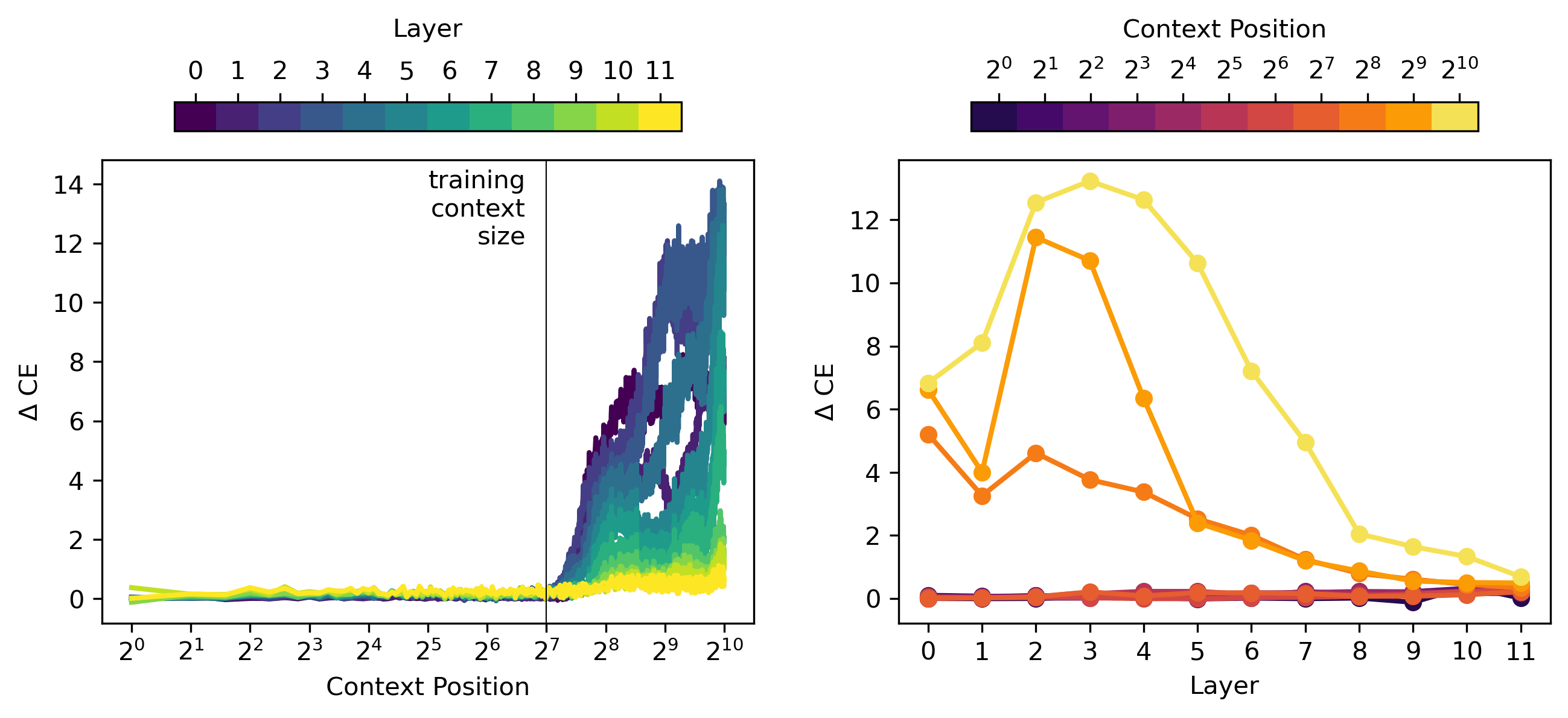
Oof, that figure does indeed suggest that, but it's because of a bug in the plot script. Thank you for pointing that out, here's a fixed version:
I've fixed the repo and I'll edit the original post shortly.
This means they're somewhat problematic for OOD use cases like treacherous turn detection or detecting misgeneralization.
I kinda want to push back on this since OOD in behavior is not obviously OOD in the activations. Misgeneralization especially might be better thought of as an OOD environment and on-distribution activations?
I think we should come back to this question when SAEs have tackled something like variable binding with SAEs. Right now it's hard to say how SAEs are going to help us understand more abstract thinking and therefore I think it's hard to say how problematic they're going to be for detecting things like a treacherous turn. I think this will depend on how how representations factor. In the ideal world, they generalize with the model's ability to generalize (Apologies for how high level / vague that idea is).
Some experiments I'd be excited to look at:
- If the SAE is trained on a subset of the training distribution, can we distinguish it being used to decompose activations on those data points off the training distribution?
- How does that compare to an SAE trained on the whole training distribution from the model, but then looking at when the model is being pushed off distribution?
I think I'm trying to get at - can we distinguish:
- Anomalous activations.
- Anomalous data points.
- Anomalous mechanisms.
Lots of great work to look forward to!
@Evan Anders "For each feature, we find all of the problems where that feature is active, and we take the two measurements of “feature goodness" <- typo?
Ah! That's the context, thanks for the clarification and for pointing out the error. Yes "problems" should say "prompts"; I'll edit the original post shortly to reflect that.
Has anyone tried training an SAE using the performance of the patched model as the loss function? I guess this would be a lot more expensive, but given that is the metric we actually care about, it seems sensible to optimise for it directly.
This is a good idea and is something we're (Apollo + MATS stream) working on atm. We're planning on releasing our agenda related to this and, of course, results whenever they're ready to share.
I've heard this idea floated a few times and am a little worried that "When a measure becomes a target, it ceases to be a good measure" will apply here. OTOH, you can directly check whether the MSE / variance explained diverges significantly so at least you can track the resulting SAE's use for decomposition. I'd be pretty surprised if an SAE trained with this objective became vastly more performant and you could check whether downstream activations of the reconstructed activations were off distribution. So overall, I'm pretty excited to see what you get!
Am I right in thinking that your ΔCE metric is equivalent to the KL Divergence between the SAE patched model and the normal model?
After seeing this comment, if I were to re-write this post, maybe it would have been better to use the KL Divergence over the simple CE metric that I used. I think they're subtly different.
Per the TL implementation for CE, I'm calculating: CE = where is the batch dimension and is context position.
So CE = for the baseline probability and the patched probability.
So this is missing a factor of to be the true KL divergence.
I think it is the same. When training next-token predictors we model the ground truth probability distribution as having probability for the actual next token and for all other tokens in the vocab. This is how the cross-entropy loss simplifies to negative log likelihood. You can see that the transformer lens implementation doesn't match the equation for cross entropy loss because it is using this simplification.
So the missing factor of would just be I think.
Oh! You're right, thanks for walking me through that, I hadn't appreciated that subtlety. Then in response to the first question: yep! CE = KL Divergence.
Could the problem with long context lengths simply be that the positional embedding cannot be represented by the SAE? You could test this by manually adding the positional embedding vector when you patch in the SAE reconstruction.
I think this is most of what the layer 0 SAE gets wrong. The layer 0 SAE just reconstructs the activations after embedding (positional + token), so the only real explanation I see for what it's getting wrong is the positional embedding.
But I'm less convinced that this explains later layer SAEs. If you look at e.g., this figure:
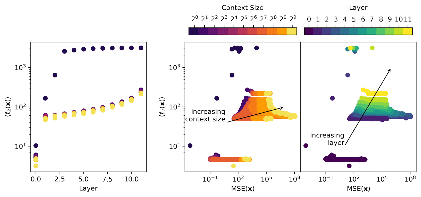
then you see that the layer 0 model activations are an order of magnitude smaller than any later-layer activations, so the positional embedding itself is only making up a really small part of the signal going into the SAE for any layer > 0 (so I'm skeptical that it's accounting for a large fraction of the large MSE that shows up there).
Regardless, this seems like a really valuable test! It would be fun to see what happens if you just feed the token embedding into the SAE and then add in the positional embedding after reconstructing the token embedding. I'd naively assume that this would go poorly -- if the SAE for layer 0 learns concepts more complex than just individual token embeddings, I think that would have to be the result of mixing positional and token embeddings?
My mental model is the encoder is working hard to find particular features and distinguish them from others (so it's doing a compressed sensing task) and that out of context it's off distribution and therefore doesn't distinguish noise properly. Positional features are likely a part of that but I'd be surprised if it was most of it.
Note: The second figure in this post originally contained a bug pointed out by @LawrenceC, which has since been fixed.
Summary
Introduction
Last year, Anthropic and EleutherAI/Lee Sharkey's MATS stream showed that sparse autoencoders (SAEs) can decompose language model activations into human-interpretable features. This has led to a significant uptick in the number of people training SAEs and analyzing models with them. However, SAEs are not perfect autoencoders and we still lack a thorough understanding of where and how they miss information. But how do we know if an SAE is “good” other than the fact that it has features we can understand?
SAEs try to reconstruct activations in language models – but they don’t do this perfectly. Imperfect activation reconstruction can lead to substantial downstream cross-entropy (CE) loss increases. Generally “good” SAEs retrieve 80-99% of the CE loss (compared to a generous baseline of zero ablation), but only retrieving 80% of the CE loss is enough to substantially degrade the performance of a model to that of a much smaller model (per scaling laws).
The second basic metric often used in SAE evaluation is the average per-token ℓ0 norm of the hidden layer of the autoencoder. Generally this is something in the range of ~10-60 in a “good” autoencoder, which means that the encoder is sparse. Since we don’t know how many features are active per token in natural language, it’s useful to at least ask how changes in ℓ0 relate to changes in SAE loss values. If high-loss data have drastically different ℓ0 from the SAE’s average performance during training, that can be evidence of either off-distribution data (compared to the training data) or some kind of data with more complex information.
The imperfect performance of SAEs on these metrics could be explained in a couple of ways:
It’s important to determine if we can understand where SAE errors come from. Distinguishing between the above worlds will help us guide our future research directions. Namely:
One way to get traction on this is to ask whether the errors induced by SAEs are random. If not, perhaps they are correlated with factors like:
If we can find results that suggest that the errors aren’t random, we can leverage correlations found in the errors. These errors can at least help us move in a direction of understanding how robust SAEs are. Perhaps these errors teach us to train better SAEs, and move us into a world where we can interpret features which reconstruct model activations with high fidelity.
In this post, we’re going to stress test the gpt2-small residual stream SAEs released by Joseph Bloom. We’ll run different random Open WebText tokens through the autoencoders and we’ll also test the encoders using the Lambada benchmark. Our biggest finding echoes Sam Marks' comments on the original post, where he preliminarily found that SAE performance degrades significantly when a context longer than the training context is used.
Experiment Overview
Open WebText next-token prediction (randomly sampled data)
Our first experiment asks how context position affects SAE performance. We pass 100k tokens from open WebText through gpt2-small using a context length of 1024. We cache residual stream activations, then reconstruct them using Joseph’s SAEs, which were trained on Open WebText using a context length of 128. We also run separate forward passes of the full gpt2-small model while intervening on a single layer in the residual stream by replacing its activations with the SAE reconstruction activations.
We measure the following quantities:
For each of these, we take means, denoted e.g., ⟨ℓ0(f)⟩. Means are taken over the batch dimension to give a per-token value.
We also examine error propagation from an SAE in an earlier layer to an SAE in a later layer. Here, we only examine context positions ≤ 100 (shorter than the training context). We replace the activations at an early layer during a forward pass of the model. We cache the downstream activations resulting from that intervention, then reconstruct those intervened-on activations with later layer SAEs.
Benchmarks (correct answer prediction)
In our second set of experiments, we take inspiration from the original gpt-2 paper. We examine the performance of gpt2-small as well as gpt2-small with SAE residual stream interventions. We examine the test split of Lambada (paper, huggingface), and in an appendix we examine the Common Noun (CN) partition of the Children’s Book Test (CBT, paper, huggingface). In both of these datasets, a prompt is provided which corresponds to a correct answer token, so here we can measure how the probability of the correct answer changes. As in the previous experiments, we also measure ℓ0, MSE, and ℓ2 – but here we average over context rather than looking per-token. We also measure Δlnp, the change in the log-probability of the model predicting the correct token.
Furthermore, we are interested in seeing whether SAE features were consistently “helpful” or “unhelpful” to the model in predicting the next answer. For each feature, we find which tokens it is active on. The mean Δlnp over all of the contexts where the feature is active is computed. We also measure a “score” for each feature, such that for every prompt where the feature is active and Δlnp≥0, it gets a +1; for every prompt where it is active and Δlnp<0, it gets a -1. We then sum this over all prompts where a feature is active to get the feature score.
How does context length affect SAE performance on randomly sampled data?
In the plot below, we show the ℓ0 norm (left panels), the average MSE reconstruction error from the SAEs (middle panels), and the SAE feature activation ℓ1 norm (right panels). The top panels are plotted vs. context position (colored by layer) and the bottom panels are plotted vs. layer (at a few context positions, colored by position at indices [1, 2, 4, 8, 16, 32, 64, 128, 256, 512, 1022] – we do not examine the 0th or last index).
The top row of plots says that all metrics follow reasonable trends for context positions ≤ 128 (the size the model was trained on) and then explode at later context positions. The bottom row shows us that early layers in the model (~layers 1-4) have much worse degradation of performance at late positions than later layers do.
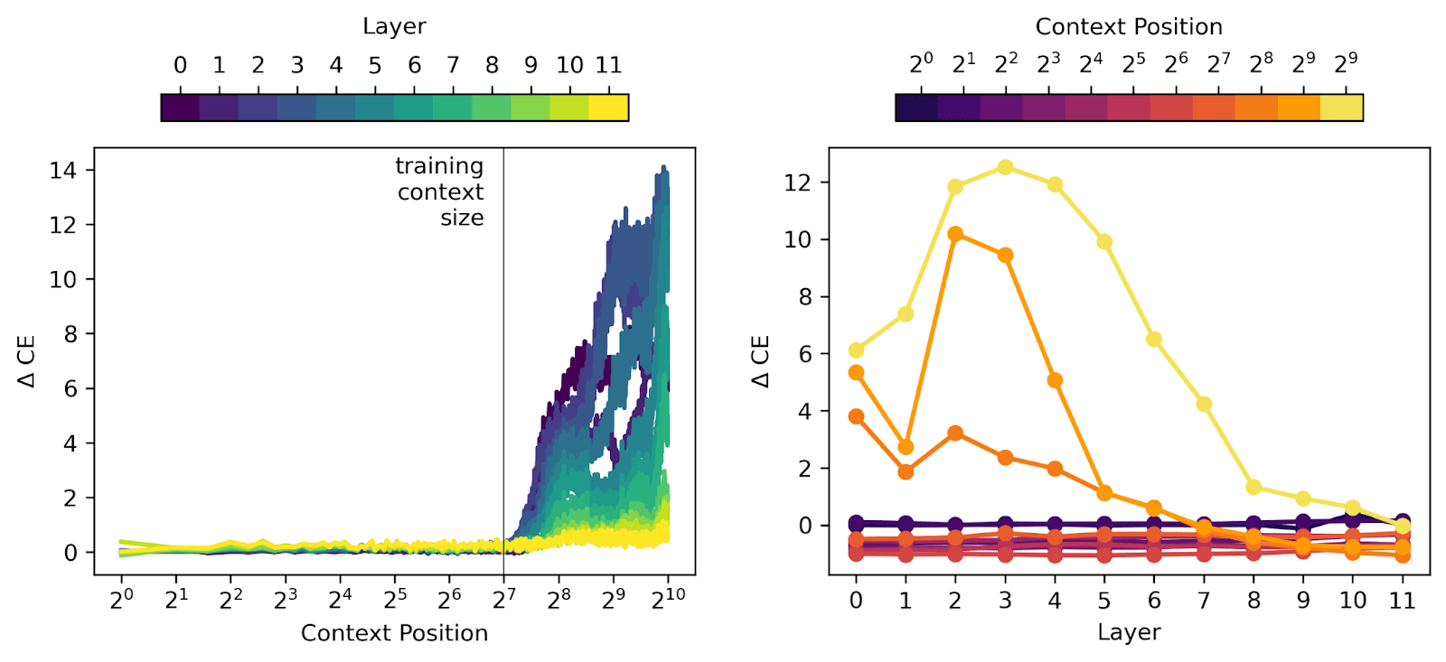
Below we see the same sort of behavior in the cross entropy (CE) loss (plotted in the same colors as the figure above). We run a forward pass and replace the chosen layer’s residual stream activations with the corresponding SAE reconstruction of those activations. We find the CE loss of this modified forward pass and subtract off the CE loss of a standard forward pass to get ΔCE.
This downstream measurement is consistent with the local measurements from the previous plot. The SAEs themselves perform poorly at context positions later than the training context, meaning that they’re not sparse and they don’t reconstruct the activations. As a result, when we replace residual stream activations with SAE outputs, the model’s ability to predict the next token is also degraded. It’s quite interesting that earlier layers of the model are increasingly susceptible to this effect!
It’s possible that the reason that the SAEs are struggling to reconstruct the residual stream contributions at later context positions is because the residual stream activations themselves come from a very different distribution. One way to examine this is to look at the average ℓ2 norm of the residual stream activations being recovered. We plot ℓ2 vs. layer in the left panel, and vs MSE in the right two panels (the right two panels are the same data with different coloring).
In the left panel, we see that later layers have larger activations (as expected through residual stream accumulation). Later positions in the context have very slightly smaller norms than earlier positions in the context (yellow points are slightly lower than darker ones they lie over). Note that the BOS token has larger activations than later tokens and must be excluded from averages and analyses. In the right panel, we see again that context size is the primary culprit of poor SAE performance (MSE), while there’s no obvious dominant trend with layer or ℓ2 norm.
Hopefully increasing the training context will fix this poor behavior we see at long contexts that we outline above.
SAE Downstream Error Propagation
We also briefly examine performance of an SAE when it tries to reconstruct activations that have already been affected by an upstream SAE intervention. We replace the activations in an early layer denoted by the x-axis in the figure below (so in the first column of the plots below, the layer 0 activations are replaced with their SAE reconstructions). We cache the downstream activations resulting from that intervention at each subsequent layer, then reconstruct the activations of each subsequent layer with an SAE (denoted by the y-axis). We specifically look at fractional changes compared to the case where there is no upstream intervention, e.g., the left plot below shows the quantity [(reconstruction MSE with upstream intervention) / (MSE reconstruction on standard residual stream) - 1]. Similar fractional changes are shown for SAE feature ℓ0 in the middle panel. The right hand panel shows how the first intervention changes the downstream residual stream ℓ2. Red colors signify larger quantities while blue signifies smaller quantities, and a value of 1 is an increase of 100%. We do not include tokens late in the context due to poor SAE performance, so this plot is an average of fractional change over the first 100 (non-BOS) tokens.
Most interventions modestly decrease downstream activation magnitudes (right panel), with the exception of layer 0 interventions increasing all downstream activation magnitudes and layer 11 typically having larger activation magnitudes after any intervention. Intervening at an early layer also tends to increase MSE loss downstream (this is a big problem for layer 9 regardless of which upstream layer is replaced, and is particularly bad for layer 3 when layer 2 is replaced). Most of these interventions also increase the ℓ0 in downstream SAEs, and perhaps this lack of sparsity provides a hint that could help explain their poorer performance. We don’t want to dwell on these results because we don’t robustly understand what they tell us, but finding places where SAEs compose poorly (e.g., layer 9) could provide hints into the sorts of features that our SAEs are failing to learn. Maybe layer 9 performs some essential function that upstream SAEs are all failing to capture.
How does using SAE output in place of activations affect model performance on the Lambada Benchmark?
Next we examined the Lambada benchmark, which is a dataset of prompts with known correct answers. In an appendix, we examine the Children’s Book Test, which has long questions where the SAEs should perform poorly. We examined 1000 questions from the test split of Lambada. A sample prompt looks like (bolded word is the answer the model has to predict):
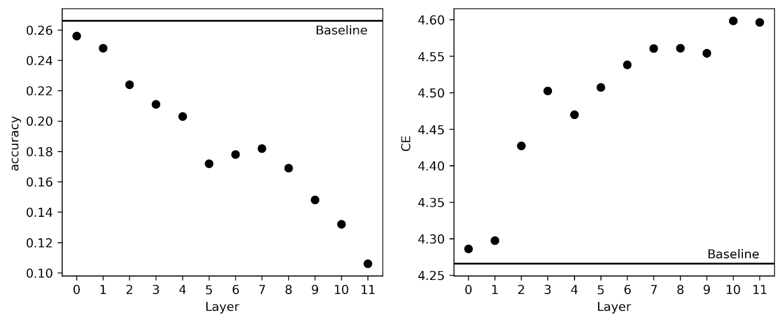
Baseline gpt2-small accuracy on these 1000 questions is 26.6%. Below we plot the downstream accuracy and average CE loss across the 1000 questions when we replace each residual stream layer with the SAE activation reconstructions.
So we see that early layers do not degrade performance much but late layers degrade performance appreciably. Interestingly, we find slightly different trends here than Joseph found for the CE loss on Open WebText in his original post – for example, there he saw that CE loss was degraded monotonically by layer until layer 11 where it improved from layer 10 a bit. Here, layer 4 has a lower CE loss than layer 3, and while layer 10 and 11 each have about the same CE, layer 11 has worse performance on Lambada than layer 10. So this sort of benchmark does seem to provide a different type of information than plain CE loss on random tokens from the training text.
Next, we examine Lambada prompts in terms of how the downstream CE loss is changed by replacing residual stream activations with SAE reconstructions. In the left panel, we plot autoencoder MSE vs ΔCE and in the right panel we plot Δlnp vs ΔCE. Data points are colored according to whether the baseline model and SAE-intervened model answered correctly. Green points are where both are correct, red are where both are incorrect, and orange and blue are where only one is correct (see legend). The upper and right-hand sub-panels show the marginal probability distributions over each class of points.
All four datapoint classes seem to share roughly the same distribution in ΔCE and in the MSE of activation reconstruction. This again demonstrates that CE loss is not a perfect proxy for model performance on the Lambada task. Unsurprisingly, the four classes do have different distributions in terms of Δlnp, which we expect because Δlnp relates directly to correctness of answer. It is interesting that there are some blue points where Δlnp<0, meaning the correct answer’s probability decreased but the intervened model answered correctly anyways. We interpret these points as being prompts where other answers which the model had preferred suffered larger decreases in probability than the correct answer did, so despite a decrease in probability, the correct answer overall became the most probable.
In the plot below, we show a layer-by-layer and a point-by-point breakdown of errors. The y-axis is Δlnp of the correct answer caused by intervening. The left panel is a strip plot showing the distribution of Δlnp layer-by-layer. The right plot is a parallel coordinate plot showing how the autoencoders respond to each datapoint, and how Δlnp from each datapoint changes as they travel through the layers of the model. In the right panel, individual prompts are colored by their y-axis value at layer 0.
In the strip plot, we see that the mean performance trends downwards layer by layer, but the layers with the most variability are the layers a few from the beginning (3) and a few from the end (9). In the right panel, we see that there is no strong prompt-level effect. SAEs introduce quasi-random errors which can increase or decrease Δlnp of the correct answer depending on the layer.
Below we plot similar plots (strip, parallel-coordinate) but for the residual stream activations which are the inputs to the SAEs.
Here we see a clear layer and prompt effect. Later layers naturally have larger activations due to accumulation of attention/MLP outputs layer-by-layer. Prompts with large activations after embedding (see colorbar) tend to have large activations throughout all layers of the model and vice versa.
We can ask how metrics of interest vary with the magnitude of input activations. To avoid looking at layer effects, we normalize the mean ℓ2 norms of residual stream activations at each layer by the minimum ℓ2 value in the dataset within that layer. Below are scatterplots of MSE (upper left), ℓ0 (upper right), ℓ1 (lower left), and Δlnp (lower right) for each datapoint and at each layer.
We first note the x-axis: each layer experiences little variance among the activations (maximum change of ~40% from the minimum value). We see no strong trends. There do seem to be weak trends in the left-hand panels: as residual stream activations grow, so too does the ℓ1 norm of the SAE, and in turn the MSE may shrink somewhat. However, there is no strong evidence in our dataset that the performance of the SAE is intricately dependent on the magnitude of residual stream inputs.
Finally we examine the performance of each of the 24k features in the SAEs at a high level. For each datapoint, over the last 32 tokens of the context, we determine which features are active (fi>0). For each feature, we find all of the prompts where that feature is active, and we take the two measurements of “feature goodness” described in the experiment overview. In the top panel, we plot a histogram of the values of the mean Δlnp achieved by each feature when they are active. In the bottom panel, we plot a binary “score” for each feature, which determines if a feature is active more often on positive Δlnp answers or negative ones.
We see the same story in the top panel as in our first strip plot: the mean of the distribution shifts to the left (worse performance) at later layers in the model. But, interestingly, all SAEs at all layers have a small distribution of features that are to the right of the black line – which means, on average, they are active when Δlnp is positive!
If we look at the bottom histogram, we see a much smaller family of features that have a positive score. This discrepancy between the top and bottom histograms means that the family of features which makes up the tail of ‘helpful’ features in the top histogram also have lots of activations where the model’s performance is weakly hurt by SAE intervention as well as a few activations where the model’s performance is strongly helped; these outliers push the mean into the positive in the top panel. Still, there is a very small family of features with positive scores, especially in early layers.
Perhaps nothing here is too surprising: model performance gets worse overall when we replace activations with SAE outputs, so the fact that most SAE features hurt model performance on a binary benchmark makes sense. We haven’t looked into any individual features in detail, but it would be interesting to investigate the small families of features that are helpful more often than not, or the features that really help the model (large Δlnp) some of the time.
Takeaways
Future work
This work raised more questions than it answered, and there’s a lot of work that we didn’t get around to in this blog post. We’d be keen to dig into the following questions, and we may or may not have the bandwidth to get around to this any time soon. If any of this sounds exciting to you, we’d be happy to collaborate!
Code
The code used to produce the analysis and plots from this post is available online in https://github.com/evanhanders/sae_validation_blogpost. See especially gpt2_small_autoencoder_benchmarks.ipynb
Acknowledgments
We thank Adam Jermyn, Logan Smith, and Neel Nanda for comments on drafts of this post which helped us improve the clarity of this post, helped us find bugs, and helped us find important results in our data. EA thanks Neel Nanda and Joseph Bloom for encouraging him to pull the research thread that led to this post. EA also thanks Stefan Heimersheim for productive conversations at EAG which helped lead to this post. Thanks to Ben Wright for suggesting we look at error propagation through layers. EA is also grateful to Adam Jermyn, Xianjung Yang, Jason Hoelscher-Obermaier, and Clement Neo for support, guidance, and mentorship during his upskilling.
Funding: EA is a KITP Postdoctoral Fellow, so this research was supported in part by grant NSF PHY-2309135 to the Kavli Institute for Theoretical Physics (KITP). JB is funded by Manifund Regrants and Private Donors, LightSpeed Grants and the Long Term Future Fund.
Compute: Use was made of computational facilities purchased with funds from the National Science Foundation (CNS-1725797) and administered by the Center for Scientific Computing (CSC). The CSC is supported by the California NanoSystems Institute and the Materials Research Science and Engineering Center (MRSEC; NSF DMR 2308708) at UC Santa Barbara. Some computations were also conducted on the RCAC Anvil Supercomputer using NSF ACCESS grant PHY230163 and we are grateful to Purdue IT research support for keeping the machine running!
Citing this post
Appendix: Children’s Book Test (CBT, Common Noun [CN] split)
As a part of this project we also looked at an additional benchmark. We chose to punt this to an appendix because a lot of the findings here are somewhat redundant with our Open WebText exploration above, but we include it for completeness.
We examine 1000 entries from the Common Noun split of the Children’s Book Text. These entries contain a 20-sentence context, and a 1-sentence fill-in-the-blank prompt. This context is long compared to what the models were trained on, so we expect the SAEs to perform fairly poorly here. An example of a CBT prompt is (bolded word is word that must be predicted):
Now let’s examine the same types of plots as we examined in the Lambada section.
Baseline gpt2-small accuracy on these 1000 questions is 41.9%. Below we plot accuracy and the average CE loss across the 1000 prompts.
Interestingly, we see the opposite trend as we saw for Lambada! For these long-context prompts, early layers manage about 0% accuracy! Later layers recover about ⅔ of the accuracy that baseline gpt2-small have, but are still quite a bit worse than baseline gpt2-small (and have significantly higher loss).
Below are scatterplot/histogram plots showing the distribution of features in MSE, ΔCE, and log-prob space.
The outlier points on the left-hand side are interesting, and seem to be out-of-distribution activations (see scatterplots below). Otherwise, there again does not seem to be a clear story between ΔCE, CBT performance, and SAE MSE.
Next, we look at the layer effect:
The middle layers (2-5) are very high-variance and add most of the noise here, and they can totally ruin the model’s ability to get the right answer (or, in edge cases, make it much much more likely!). In the right-hand plot, there’s no strong prompt-level effect, but it seems like there might be something worth digging into further here. The gradient of light (at the bottom) to dark (at the top) seems more consistent than it did for the Lambada test above.
Residual stream activations follow a rather different trend than the Lambada ones did (and this involves no SAE intervention!):
The intermediate layers have a huge amount of variance in the residual stream magnitudes, and later layers can have smaller residual stream norms than layer 2. This is very counter-intuitive, and it must mean that early layers are outputting vectors into the residual stream which later layers are canceling out.
Next we look at scatter plots again:
There seem to be some trends here. At each layer, there is a ‘hook’ effect, where low-norm activations show a trend, in all but the bottom left panel, then there is a hook, and the trend changes. Strangely, the only layer where activations monotonically increase with input activation strength is layer 1; all other layers have a maximum MSE error at a lower activation strength and an overturning (MSE decreasing with input activation norm).
Another interesting distribution here: layers ~2-5 have a cloud of data points with very high ℓ2 activations and very low downstream Δlnp! So despite the interesting trends seen in MSE, replacing model activations with SAE activations when the original residual stream has a large norm harms the model’s ability to correctly predict the answer token. It’s unclear if these high norm prompts are somehow out-of-distribution compared to the text corpus that gpt2-small and the SAEs were trained on.
Finally, we look at feature histograms:
While there are again a few features which lead to large (positive) Δlnp, and thus there are a few features to the right of the 0 line in the top panel, there are zero features which are, on average, active only when the model’s probability of guessing correctly is improved. Interestingly, there are a few features in the layer 0 encoder which are almost always active and the model never sees an improvement when they’re active.