Also, finite factored sets are a really neat mathematical structure: they are a way of taking a set and expressing it as a productof some factors. Set factorizations are analogous to integer factorizations, in the same way that set partitions are analogous to integer partitions.
So, here is my current understanding of finite factored sets, in pictures.
1. What are Set Factorizations?
What do these “factored sets” look like? Let’s start with a set S and factor it.
The first concept we need is a partition of a set S. A partition is a way of chopping up S into subsets (called parts). Here are a few examples of partitions:
We usually call the partitions X,Y,Z,U,V, or W, and their parts xi,yi,… like this:
U is called the trivial partition. It only has one part.
We can think of partitions as properties, or variables over our set. For example, consider a set like this:
and compare it to the partitions X,Y and Z from above:
Then
The partition X is the property “color”, with x1 = blue and x2 = orange.
The partition Y is the property “form” with y1 = square, and y2 = circle.
The partition Z is the property “filled” with z1 = yes, and z2 = no.
Exercise
Consider these two partitions X and Y on the set S. What would it look like to represent them as properties (e.g. X = shape, Y = color) instead?
Spoiler space
It could look something like this:
Here X = shape = {x1,x2,x3} = {star, circle, square}, and Y = color ={y1,y2} = {green, orange}.
I hope you can see how partitions and properties are basically the same thing. In the rest of this post, I will use “partitions” and “properties” interchangeably. Sometimes I will use the ring-style visualization of partitions, and sometimes the property style, depending on what I find more intuitive in any given example.
Now we can define set factorizations:
A factorization B of our set S looks like this:
A factorization is a set B={b1,b2,…,bn} of partitions (called factors). In this case B={b1,b2}={X,Y}={{x1,x2},{y1,y2}}.
But it can’t just be any set of partitions. In the following sections, I will explain the two conditions that B needs to fulfill in order to count as a factorization:
There is a unique element for all combinations of properties
No factor is trivial
1. There is a unique element for all combinations of properties
Let’s look at our partitions in terms of properties again:
What we need in order for B to be a factorization, is that for all combinations(xi,yj) of properties (for example (x1,y2), which is (blue, circle)), there is a unique element with these properties.
We can see that this is the case here: We have exactly one blue square, exactly one orange square, exactly one blue circle, and exactly one orange circle.
To express it more mathematically: For B={X1,X2,…,Xn} to be a factorization, we need that for all x1∈X1,x2∈X2,…xn∈Xn, it holds that the intersection of {x1,x2,…,xn} contains exactly one element. This means the cartesian product of our factors is bijective to the set S, which justifies that we say we can “express S as the product of our factors”.
2. No factor is trivial
Here is an example of a non-factorization:
B = {U, V} is not a factorization here, because U is trivial and factors aren’t allowed to be trivial.
This is analogous to integer factorization, where we don’t count 1 as a factor. For example, for the integer 6 we say the factorizations are {6} and {2,3}, and don’t mention {6,1} and {6,1,1} and {6,1,1,1} and so on.
Exercise
What about this? Is B = {X, Y} a factorization here? (take a moment to think for yourself)
more spoiler space
… No. B is not a factorization.
Why not? Let’s look at it in terms of properties again:
We can see that there is not a unique element for every combination of properties. For example, there is no orange star, and also no orange circle (i.e. x1∩y2 and x2∩y2 are empty).
What about this one? Is B = {V} a factorization?
… yes it is. This one is called trivial factorization. Each set can be factorized as B={b1} with b1 being the maximally separating partition.
If you play around a bit with sets of different sizes, you will see that the possible set factorizations correspond to the integer factorizations of the set’s size [1]:
In particular, sets with a prime number of elements only have the trivial factorization.
This concludes the examples for factorizations. Hopefully you now have some grasp on how factoring a set works.
If we have a tuple F = (S, B) of a set S and a factorization B of S, then we call F a factored set. In this post I will assume that all sets are finite, and use “factored set” synonymously with “finite factored set”
2. What does this have to do with Causality? - The Building Blocks
In this section, I will introduce three building blocks: three structures on factored sets, that will help us make the connection to causality later.
In section 3, I will then use these building blocks to model the causal structure behind a probability distribution with factored sets, similar to causal graphs.
The three building blocks are:
The history of a partition X is related to a random variable’s set of ancestors in a causal graph
Orthogonality of two partitions X, Y means they have no shared history. In the Pearl-paradigm we know that two variables X and Y have no common ancestors if and only if they are independent. Analogously, Scott Garrabrant proved that in the factored set paradigm, two variables are orthogonal if and only if they are independent. [2]
Conditional orthogonality of two partitions: In the Pearl-paradigm we know that two variables X and Y are d-separated if and only if they are conditionally independent (proof here and here). Analogously, Scott proved that in the factored set paradigm, two variables are conditionally orthogonal if and only if they are conditionally independent. [2]
"Time": Saying a partition A is before B is related to a causal path going from A to B in a causal graph.
History
Consider an 8-element set S, which is factorized into the factors “color”, “shape” and “fill”, like this:
Here, the factored set F is F = (S, B) with the factorization B = {color, shape, fill}.
Now, let’s consider a partition/property A - which does not need to be a factor! (i.e. A does not have to be color, shape or fill here):
Now assume we know some properties of an element s, and want to figure out if it is in a1 or in a2. The fill doesn’t matter for this, so the minimum required properties for finding out are {color, shape}.
If we know that the color is blue, then the color would be enough to determine that we are in a2, but in order to reliably find out if we are in a2, we need both color and shape.
This is what we will call the history of A: We say that in a factored set F, the history hF(A) of a property A is the set of properties we need in order to figure out A.
Once we build up factored sets as a model for a causal structure, the history of a partition A will correspond to the set of ancestors of a random variable in a causal graph.
Note that I represent A as these red rings, and {color, shape, fill} as properties. I could just as well represent A as a property too (e.g. different sizes), but I prefer this representation because it distinguishes the factors in our factorization {color, shape, fill} from the variable A whose history we want to find.
Exercise
The history hF(A) of a property A is the set of properties we need in order to figure out A. So, what is the hF(A) here?
hF(A) = {color}
You only need to know the color in order to tell if an element is in a1 or in a2.
Notice that in this case, A = color. So hF(A)= {color} is the same as hF(color) = {color}. Which is basically just saying that you just need to know the color in order to find out the color. In general, for every factor b in our factorization, it holds that hF(b)={b}.
Another exercise: What if A is the trivial partition? What is hF(A) here?
Here, the history is empty! (hF(A)=∅) We don’t need to know any properties, because we alreadyknow that every s is in a1.
Orthogonality
Now we have defined history, we can define orthogonality, which is closely related to independence of random variables!
We say that two partitions A, B are orthogonal, if their histories don’t overlap.
Exercise
Are A and B orthogonal here?
No. The history of A is hF(A) = {color, shape}. The history of B is hF(B)= {color, fill}, so the histories overlap.
In the Pearl-paradigm we know that two variables X and Y have no common ancestors if and only if they are independent. Analogously, Scott Garrabrant proved that when we use a factored set to model causal structure (I’ll explain how to do that in section 3), then two variables are orthogonal if and only if they are independent. [2]
Note that in any factorization, the factors are all orthogonal to each other, because hF(b) ={b} for any factor b (we only need color to infer color, remember) so hF(b1)∩hF(b2)=∅ if b1≠b2.
Scott also defines conditional orthogonality as an analog of d-separation. I won’t define conditional orthogonality here in order to keep things simple, but you can find the definition here.
In the Pearl-paradigm there is a theorem called soundness and completeness of d-separation: Two variables X and Y are d-separated with regard to a set of variables Z if and only if X and Y are conditionally independent given Z (proof here and here)
Two variables X, Y are conditionally orthogonal with regard to a set of variables Z if and only if X and Y are conditionally independent given Z. (Technically it’s slightly more complicated, but this is the gist [2])
"Time"
We say that a partition A is weakly before B if A's history of A is a subset or equal to B's history (i.e. hF(A)⊆hF(B) ).
We say that A is strictly before B if A's history is a strict subset of B's history (i.e. hF(A)⊊hF(B)).
This notion of “time” is closely related to the concept of a causal arrow going from A to B in a causal graph.
You can imagine A's history like "everything that comes before A in time", so if everything that’s in A’s history is also in B’s history then A is before B:
Exercise
Is A or B weakly or strictly before the other here? (i.e. is one of the histories of A or B a subset of the other? Reminder: history = set of properties needed to infer our partition)
A is strictly before B! hF(A) = {color, shape} and hF(B) = {color, shape, fill}, so hF(A)⊊hF(B).
Now we have the building blocks to use factored sets for causal inference!
3. Causal Inference using Factored Sets
In this section I will walk through an example of inferring causality from data using factored sets.
Consider an experiment in which we collect 2 bits. The distribution P looks like this:
P(00) = 1% P(01) = 9% P(10) = 81% P(11) = 9%
Let’s say X is the first bit, and Y is the second bit.
In the causal graph paradigm, we would observe that X and Y are dependent (P(X=0)=10%≠P(X=0|Y=0)=182). Thus we are not able to distinguish between these three causal graphs:
We don’t know whether X causes Y, Y causes X, or there is some common factor W that causes both.
How do we look at this in the Factored Set Paradigm?
In the factored set paradigm, start with the sample space Ω of our distribution P:
We then say a model of the distribution is a factored set F = (S, B) and a function f:S→Ω:
XS and YS are the “preimages” of X and Y under f. By that I mean that all their parts xSi and ySj are the preimages of xi and yj respectively, under f. That looks as follows:
(Note that in this case f is bijective, but in general f does not have to be bijective. If we allow f to be non-bijective, then the framework works in more generality because we can describe some processes that we couldn’t otherwise describe. [3])
However, we can’t just use any factorization B. In order for (F, f) to count as a model of our distribution P, it needs to be such that the dependencies and independencies of our distribution are represented in the factorization.
That means:
Two variables X and Y are independent in P if and only if XS and YS are orthogonal in F (i.e. their histories don’t overlap)
Two variables X and Y are dependent in P if and only if XS and YS are not orthogonal in F
Remember, our probability distribution P was
P(00) = 1% P(01) = 9% P(10) = 81% P(11) = 9%
Is the following actually a model of P?
No, it is not: X, and Y are dependent in P, but XS and YS are orthogonal in F! (Note that orthogonality depends on what model we are in/what factorization we use.)
Here is a really tricky one: Is this a model of P?
Also no, but this is hard to see, so let’s walk through it.
Consider the variable Z = X XOR Y
We don’t have to express our distribution in terms of X and Y, we can just as well define it in terms of X and Z. And then it looks like this:
We can see that Z and X are independent! (becauseP(Z=0)=1%+9%=10%, and alsoP(Z=0|X=0)=1%9%+1%=10% , andP(Z=0|X=1)=9%81%+9%=10%)
What does this mean for our model? It means that ZS and XS need to be orthogonal.
Are ZS and XS orthogonal in our model? Here it is again:
No, because the history for both XS and ZS is {V}, so XS and ZS have an overlapping history.
So F = (S, {VS}) is also not a model of P.
Does our distribution P have a model at all? Yes - here is a model that actually works for P:
Here hF(XS)={XS} and hF(ZS)= {ZS}, and hF(YS) = {XS,ZS}.
This means XS and ZS are orthogonal, which matches our observation that X and Z are independent in P. Also XS and YS are not orthogonal, which matches our observation that X and Y are dependent in P.
It also means that hF(XS)⊊hF(YS), so XS is strictly before YS.
If XS is strictly before YS, then the causal arrow goes from X to Y, so we have found a causal direction! It’s this one:
From what we know so far, this causal direction X→Y only holds for this particular model (F, f), but in fact, you can also prove that X→Y holds for any model of this distribution P.
So, we just inferred causality from observational (as opposed to interventional) data, in a way that Pearl’s causal models wouldn’t have inferred!
Sanity-checking the result in Pearl’s paradigm
I have encountered a lot of skepticism that we can infer the causality X→Y here. So I’m going to switch back to the Pearl paradigm, and explain why X causes Y if our distribution is P, and we can actually infer that from only observational data without needing interventional data.
This section will assume you know how to determine (in-)dependence in probability distributions and in causal graphs. (If you don’t, you can either just believe me, or learn about it here and here).
Again, say X is the first bit, Y is the second bit, and Z = X XOR Y. Here is our distribution again, in table-form:
X
Y
Z
P(X, Y, Z)
0
0
0
1%
0
1
1
9%
1
0
1
81%
1
1
0
9%
Any other combination of X, Y, and Z
0%
The (in-)dependencies we can read from this are:
X and Y are dependent
X and Z are independent
Y and Z are dependent
The possible causal graphs which fulfill these dependencies and independencies are these four:
So, we know that Y does not cause X! This matches our finite factored set finding that X causes Y, but it's weaker. Can we also infer that X causes Y?
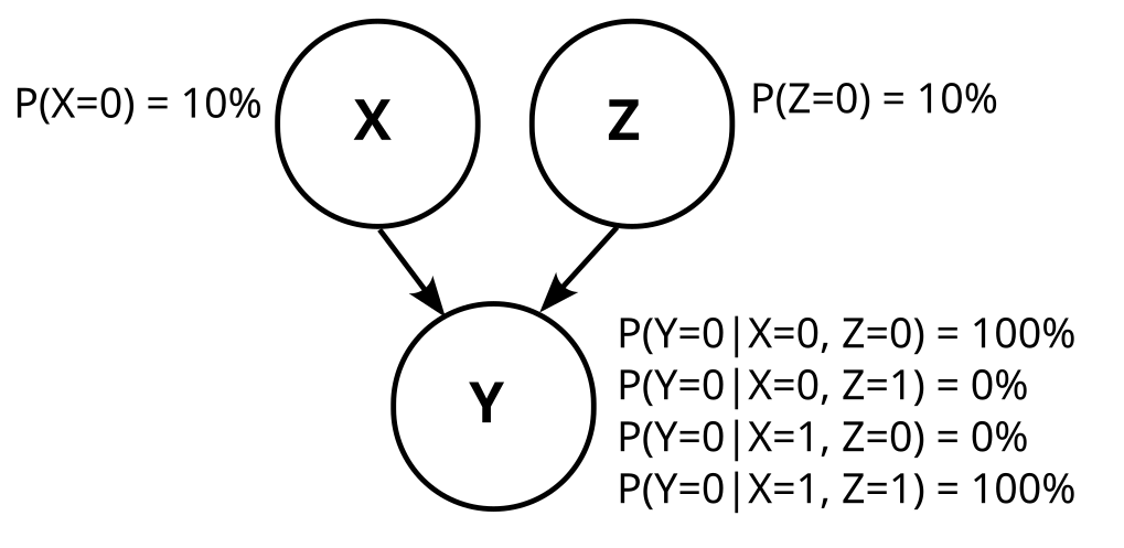
Let’s concretize the above graphs by adding the conditional probabilities. Graph 1 then looks like this:
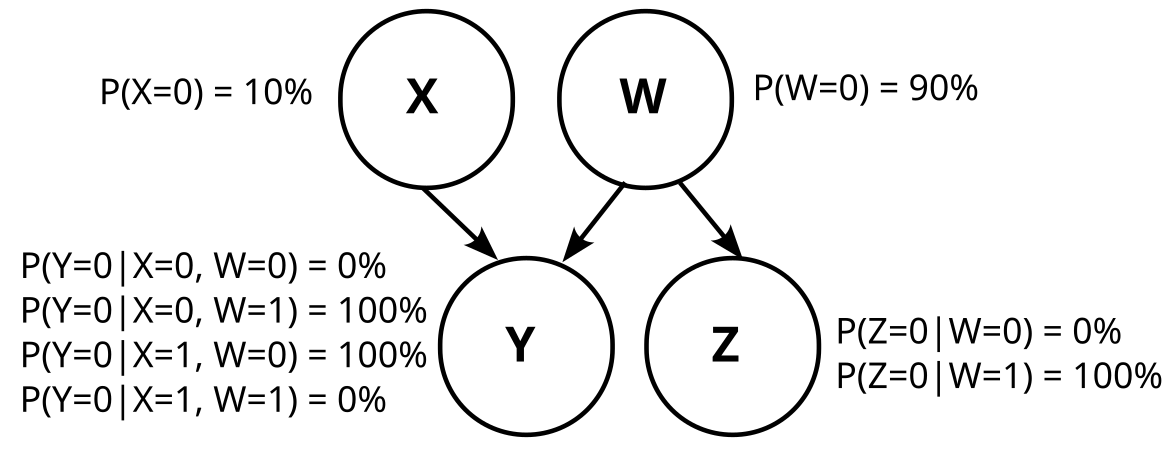
Graph 2 is somewhat trickier, because W is not uniquely determined. But one possibility is like this:
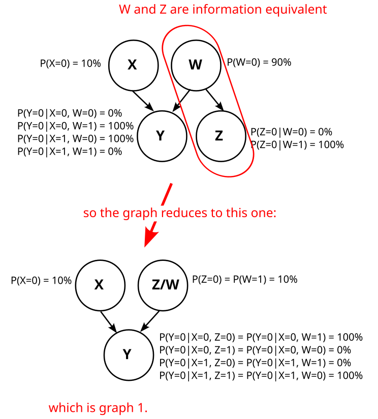
Note that W is just the negation of Z here (W=¬Z). Thus, W and Z are information equivalent, and that means graph 2 is actually just graph 1.
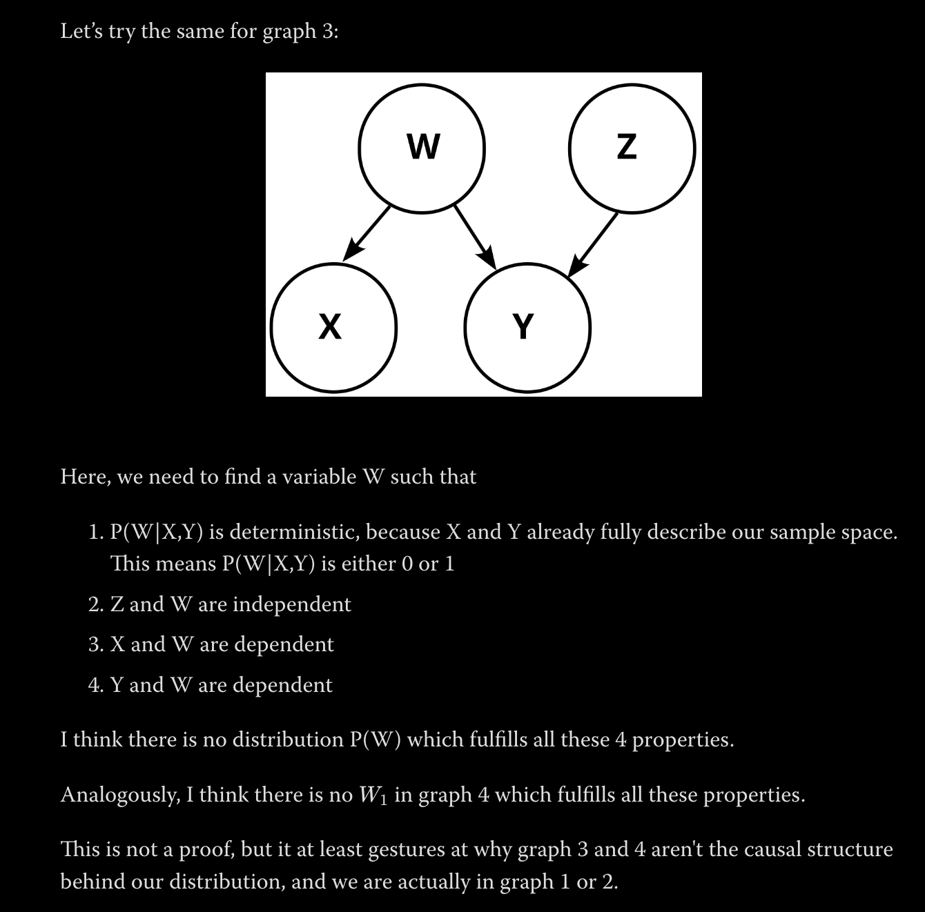
Can we find a different variable W such that graph 2 does not reduce to graph 1? I.e. can we find a variable W such that Z is not deterministic given W?
No, we can’t. To see that, consider the distribution P(Z|X,Y,W). By definition of Z, we know that
P(Z|X,Y,W)={1if Z=X XOR Y,0otherwise..
In other words, P(Z|X,Y,W) is deterministic.
We also know that W d-separates Z from X,Y in graph 2:
This d-separation implies that Z is independent from X, Z given W:
P(Z|W)=P(Z|W,X,Y)
As P(Z|X,Y,W) is deterministic, P(Z|W) also has to be deterministic.
So, graph 2 always reduces to graph 1, no matter how we choose W. Analogously, graph 3 and graph 4 also reduce to graph 1, and we know that our causal structure is graph 1:
Which means we also know that X causes Y.
The reason why we usually wouldn’t have found this causal direction using causal graphs is that we wouldn’t even have considered Z as potentially interesting. This is what factored sets give us: They make us consider every possible way of defining variables, so we don’t miss out on any information that may be hidden if we just look at a predetermined set of variables.
Summary
Set factorizations are a way of expressing sets as a product of some factors, similar to how integer factorization is about expressing integers as a product of some factors.
We can define a history on them, that tells us which properties came“before”other properties. We say that two variables are orthogonal if they have no shared history. Using these notions of history and orthogonality, we can define a mathematical structure called model of a probability distribution. With this model, we can do causal inference (inferring causal structure from data).
Factored sets let us infer causal relations that we usually wouldn’t have found using causal graphs. For example, if we have two binary variables X and Y, and X is independent from X XOR Y, then we can infer the causal direction X→Y.
Further Reading
I hope you got a bit of a grasp on finite factored sets, and see why they are really neat. If you want to read more, the best entry point is probably this edited transcript from a talk by Scott Garrabrant.
For a non-mathematical intuition how Scott relates the concepts of time, causality, abstraction, and agency, see his Saving Time post.
I haven’t looked closely into AI alignment specific applications of factored sets, but it looks like they can be used to better talk about embedded agency, decision theory, and ELK.
_____
This post is a result of a distillation workshop led by John Wentworth at SERI MATS. I’d like to thank Leon Lang, Scott Garrabrant, Matt MacDermott, Jesse Hoogland, and Marius Hobbhahn for feedback and discussions on this post.
Note that the number of set factorizations of an n-element set is not the same as the number of integer factorizations of n, because elements are distinguishable, so for example these two factorizations do not count as the same factorization:
Actually, it’s somewhat more complicated than “X and Y are (conditionally) orthogonal if and only if they are independent”. The full version is more like “If XS and YS are partitions on a set S, which has a mapping f:S→Ω to the sample space, then XS and YS are (conditionally) orthogonal if and only if the images X and Y of XS and YS are (conditionally) independent”. But for the sake of this explanation, if you just remember that “orthogonality ⇔ independence”, that's enough.
Even if f is not bijective, the “preimages” XS and YS of X and Y are always well-defined partitions. Here are two examples in which f is not bijective:
I am still confused about how you can tell the causal direction from just the raw data. Taking your toy example I could write a code that first randomly determines Y, and then decides on X, in such a way so that the probability table you give is produced. Presumably you mean something more specific by causal direction than I am imagining?
I got interested and wrote my python example. I get (up to some noise) the same distribution, and at least in my layperson way of looking at it I would say that Y has a causal effect on X.
import random
rand = random.random
def get_xy(): # Determine Y first, make it causally effect X if rand() > 82/100: Y = 1 else: Y = 0 # end if
if Y == 1: if rand() > 1/2: X = 1 else: X = 0 # end sub-if else: if rand() > 1/82: X = 1 # When Y=0 it is very likely X=1. else: X = 0 # end sub-if # end if return X, Y
dat = [0, 0, 0, 0] for _ in range(1000000): X, Y = get_xy() dat[X + 2*Y] += 1
This is a very good point, and you are right - Y causes X here, and we still get the stated distribution. The reason that we rule this case out is that the set of probability distributions in which Y causes X is a null set, i.e. it has measure zero.
If we assume the graph Y->X, and generate the data by choosing Y first and then X, like you did in your code - then it depends on the exact values of P(X|Y) whether X⊥Z holds. If the values of P(X|Y) change just slightly, then X⊥Z won't hold anymore. So given that our graph is Y->X, it's really unlikely (It will happen almost never) that we get a distribution in which X⊥Z holds. But as we did observe such a distribution with X⊥Z , we infer that the graph is not Y->X.
In contrast, if we assume the graph as X-> Y <-Z , then X⊥Z will hold for any distribution that works with our graph, no matter what the exact values of P(Y|X) are (as long as they correspond to the graph, which includes satisfying X⊥Z)
Thank you very much. That explains a lot. To repeat in my own words for my understanding: In my example perturbing any of the probabilities, even slightly, would upset the independence of Z and X. So in some sense their independence is a fine tuned coincidence, engineered by the choice of values. The model assumes that when independences are seen they are not coincidences in this way, but arise from the causal structure itself. And this assumption leads to the conclusion that X comes before Y.
I'm not quite convinced by this response. Would it be possible to formalize "set of probability distributions in which Y causes X is a null set, i.e. it has measure zero."?
It is true that if the graph was (Y->X, X->Z, Y->Z), then we would violate faithfulness. There are results that show that under some assumptions, faithfulness is only violated with probability 0. But those assumptions do not seem to hold in this example.
Would it be possible to formalize "set of probability distributions in which Y causes X is a null set, i.e. it has measure zero."?
We are looking at the space of conditional probability table (CPT) parametrizations in which the indepencies of our given joint probability distribution (JPD) hold.
If Y causes X, the independencies of our JPD only hold for a specific combination of conditional probabilities. Namely those in which P(X,Z) = P(X)P(Z). The set of CPT parametrizations with P(X,Z) = P(X)P(Z) has measure zero (it is lower-dimensional than the space of all CPT parametrizations).
In contrast, any CPT parametrization of graph 1 would fulfill the independencies of our given JPD. So the set of CPT parametrizations in which our independencies hold has a non-zero measure.
There are results that show that under some assumptions, faithfulness is only violated with probability 0. But those assumptions do not seem to hold in this example.
Could you say what these assumptions are that don't hold here?
For example, in theorem 3.2 in Causation, Prediction, and Search, we have a result that says that faithfulness holds with probability 1 if we have a linear model with coefficients drawn randomly from distributions with positive densities.
It is not clear to me why we should expect faithfulness to hold in a situation like this, where Z is constructed from other variables with a particular purpose in mind.
Consider the graph Y<-X->Z. If I set Y:=X and Z:=X, we have that X⊥Y|Z, violating faithfulness. How are you sure that you don't violate faithfulness by constructing Z?
Consider the graph Y<-X->Z. If I set Y:=X and Z:=X
I would say then the graph is reduced to the graph with just one node, namely X. And faithfulness is not violated because we wouldn't expect X⊥X|X to hold.
In contrast, the graph X-> Y <- Z does not reduce straightforwardly even though Y is deterministic given X and Z, because there are no two variables which are information equivalent.
I'm not completely sure though if it reduces in a different way, because Y and {X, Z} are information equivalent (just like X and {Y,Z}, as well as Z and {X,Y}). And I agree that the conditions for theorem 3.2. aren't fulfilled in this case. Intuitively I'd still say X-> Y <- Z doesn't reduce, but I'd probably need to go through this paper more closely in order to be sure.
Finally got around to looking at this. I didn't read the paper carefully, so I may have missed something, but I could not find anything that makes me more at ease with this conclusion.
Ben has already shown that it is perfectly possible that Y causes X. If this is somehow less likely that X causes Y, this is exactly what needs to be made precise. If faithfulness is the assumption that makes this work, then we need to show that faithfulness is a reasonable assumption in this example. It seems that this work has not been done?
If we can find the precise and reasonable assumptions that exclude that Y causes X, that would be super interesting.
Curated. I am excited about many more distillations and expositions of relevant math on the Alignment Forum. There are a lot of things I like about this post as a distillation:
Exercises throughout. They felt like they were simple enough that they helped me internalise definitions without disrupting the flow of reading.
Pictures! This post made me start thinking of finite factorisations as hyperrectangles, and histories as dimensions that a property does not extend fully along.
Clear links from Finite Factored Sets to Pearl. I think these are roughly the same links made in the original, but they felt clearer and more orienting here.
Highlighting which of Scott's results are the "main" results (even more than the "Fundamental Theorem" name already did).
Magdalena Wache's engagement in the comments.
I do think the pictures became less helpful to me towards the end, and I thus have worse intuitions about the causal inference part. I'm also not sure about the emphasis of this post on causal rather than temporal inference. But I still love the post overall.
P(W|X,Y) is deterministic, because X and Y already fully describe our sample space. This means P(W|X,Y) is either 0 or 1
Z and W are independent
X and W are dependent
Y and W are dependent
I think your arguments in Section 3 to rule out Graph 3 can't be correct if you accept Graph 2.
To see this, note that there is a symmetry between X and Z. Namely, if we use FFS temporal inference, then we know that X and Z are both before Y (and ¬Y ).(here we even have P(X=x,Z=z)=P(X=z,Z=x), so they are entirely exchangeable).
Therefore, if you accept Graph 2 then we can clearly switch X and Z in Graph 2 and obtain a solution for Graph 3. Also, note that in these solutions X=¬W or Z=¬W, so if we see variables as their information content, as in FFS, this is Graph 1 in disguise.
Also in Graph 2 there is a typo P(W=0|Z=0) instead of P(Z=0|W=0)
I don't understand why 1 is true – in general, couldn't the variable $W$ be defined on a more refined sample space? Also, I think all $4$ conditions are technically satisfied if you set $W=X$ (or well, maybe it's better to think of it as a copy of $X$).
I think the following argument works though. Note that the distribution of $X$ given $(Z,Y,W)$ is just the deterministic distribution $X=Y \xor Z$ (this follows from the definition of Z). By the structure of the causal graph, the distribution of $X$ given $(Z,Y,W)$ must be the same as the distribution of $X$ given just $W$. Therefore, the distribution of $X$ given $W$ is deterministic. I strongly guess that a deterministic connection is directly ruled out by one of Pearl's inference rules.
I agree that 1. is unjustified (and would cause lots of problems for graphical causal models if it was).
Further, I’m pretty sure the result is not “X has to cause Y” but “this distribution has measure 0 WRT lebesgue in models where X does not cause Y” (and deterministic relationships satisfy this)
Finally, you can enable markdown comments on account settings (I believe)
Further, I’m pretty sure the result is not “X has to cause Y” but “this distribution has measure 0 WRT lebesgue in models where X does not cause Y”
Yes that's true. Going from "The distributions in which X does not cause Y have measure zero" to "X causes Y" is I think common and seems intuitively valid to me. For example the soundness and completeness of d-separation also only holds but for a set of distributions of measure zero.
I think this could be right, but I also think this attitude is a bit too careless. Conditional independence in the first place has lebesgue measure 0. I have some sympathy for considering something along the lines of "when your posterior concentrates on conditional independence, the causal relationships are the ones that don't concentrate on a priori measure 0 sets" as a definition of causal direction - maybe this is implied by the finite factored set definition if you supply an additional rule for determining priors, I'm not sure.
Also, this is totally not the Pearlian definition! I made it up.
I agree with you regarding 0 lebesgue. My impression is that the Pearl paradigm has some [statistics -> causal graph] inference rules which basically do the job of ruling out causal graphs for which having certain properties seen in the data has 0 lebesgue measure. (The inference from two variables being independent to them having no common ancestors in the underlying causal graph, stated earlier in the post, is also of this kind.) So I think it's correct to say "X has to cause Y", where this is understood as a valid inference inside the Pearl (or Garrabrant) paradigm. (But also, updating pretty close to "X has to cause Y" is correct for a Bayesian with reasonable priors about the underlying causal graphs.)
(epistemic position: I haven't read most of the relevant material in much detail)
I agree that 1. is unjustified (and would cause lots of problems for graphical causal models if it was).
Interesting, why is that? For any of the outcomes (i.e. 00, 01, 10, and 11), P(W|X,Y) is either 0 or 1 for any variable W that we can observe. So W is deterministic given X and Y for our purposes, right?
If not, do you have an example for a variable W where that's not the case?
I think W does not have to be a variable which we can observe, i.e. it is not necessarily the case that we can deterministically infer the value of W from the values of X and Y. For example, let's say the two binary variables we observe are X=[whether smoke is coming out of the kitchen window of a given house] and Y=[whether screams are emanating from the house]. We'd intuitively want to consider a causal model where W=[whether the house is on fire] is causing both, but in a way that makes all triples of variable values have nonzero probability (which is true for these variables in practice). This is impossible if we require W to be deterministic once (X,Y) is known.
I see! You are right, then my argument wasn't correct! I edited the post partially based on your argument above. New version:
Can we also infer that X causes Y?
Let’s concretize the above graphs by adding the conditional probabilities. Graph 1 then looks like this:
Graph 2 is somewhat trickier, because W is not uniquely determined. But one possibility is like this:
Note that W is just the negation of Z here (W=¬Z). Thus, W and Z are information equivalent, and that means graph 2 is actually just graph 1.
Can we find a different variable W such that graph 2 does not reduce to graph 1? I.e. can we find a variable W such that Z is not deterministic given W?
No, we can’t. To see that, consider the distribution P(Z|X,Y,W). By definition of Z, we know that
P(Z|X,Y,W)={1if Z=X XOR Y,0otherwise..
In other words, P(Z|X,Y,W) is deterministic.
We also know that W d-separates Z from X,Y in graph 2:
This d-separation implies that Z is independent from X, Z given W:
P(Z|W)=P(Z|W,X,Y)
As P(Z|X,Y,W) is deterministic, P(Z|W) also has to be deterministic.
So, graph 2 always reduces to graph 1, no matter how we choose W. Analogously, graph 3 and graph 4 also reduce to graph 1, and we know that our causal structure is graph 1:
I basically agree with this: ruling out unobserved variables is an unusual way to use causal graphical models.
Also, taking the set of variables that are allowed to be in the graph to be the set of variables defined on a given sample space makes the notion of "intervention" more difficult to parse (what happens to F:=(X,Y) after you intervene on X?), though it might be possible with cyclic causal relationships.
So basically, "causal variables" in acyclic graphical models are neither a subset nor a superset of observed random variables.
What does the ⊊ symbol mean? I understand the basics of set notation but haven't taken a class, and I haven't been able to find this symbol on the tables of set notation I've looked at.
Strict subset - that is, the set on the left is contained in the set in the right, but the set in the right as at least one item not contained in the set on the left.
Possibly! Extending factored sets to continuous variables is an active area of research.
Scott Garrabrant has found 3 different ways to extend the orthogonality and time definitions to infinite sets, and it is not clear which one captures most of what we want to talk about.
I suspect that the fundamental theorem can be extended to finite-dimensional factored sets (i.e., factored sets where |B| is finite), but it can not be extended to arbitrary-dimension factored sets
If his suspicion is right, that means we can use factored sets to model continuous variables, but not model a continuous set of variables (e.g. we could model the position of a point in space as a continuous random variable, but couldn't model a curve consisting of uncountably many points)
Sorry if I'm goofing up here, but I got confused about the math. You in "How do we look at this in the Factored Set Paradigm," you say that P(Z=0) = (1%+9%)/(81%+9%) = 1/9 = 11.111...%
It seems like P(Z=0) is actually (1%+9%)/(1%+9%+81%+9%) = 10%. Am I misreading something here?
I think you're correct that P(Z=0) is 1/10 -- the author seems to have been calculating the odds ratio instead of the probability. (In fact, they correctly say that P(Z=0) is 1/10 later on in the post).
The reason why we usually wouldn’t have found this causal direction using causal graphs is that we wouldn’t even have considered Z as potentially interesting. This is what factored sets give us: They make us consider every possible way of defining variables, so we don’t miss out on any information that may be hidden if we just look at a predetermined set of variables.
I don't quite understand how this conclusion is reached. Referring to the previous section:
Yes - here is a model that actually works for P:
What is the procedure by which we identify the particular set factorization that models our distribution? Is this identification in some meaningful sense easier than guessing Z directly? I'm just confused about what has been gained here.
What is the procedure by which we identify the particular set factorization that models our distribution?
There is not just one factored set which models the distribution, but infinitely many. The depicted model is just a prototypical example.
The procedure for finding causal relationships (e.g. X→Y in our case) is not trivial. In that part of his post, Scott sounds like it's
1. have the suspicion that X→Y 2. prove it using the histories
I think there is probably a formalized procedure to find causal relationships using factored sets, but I'm not sure if it's written up somewhere.
For causal graphs, I don't know if there is a formalized procedure to find causal relationships which take into account all possible ways to define variables on the sample space. My general impression is that causal graphs become pretty unwieldy once we introduce deterministic nodes. And then many rules we usually use with causal graphs don't hold anymore, and working with graphs then becomes really unintuitive.
So my intuition is that yes, finding causal relationships while taking into account all possible ways to define variables is easier with factored sets than with causal graphs. (And I'm not even sure if it's even possible in general with causal graphs.) But my intuition on this isn't based on knowing a formal procedure for finding causal relationships, it just comes from my impression when playing around with the two different representations.
Finite factored sets are a new paradigm for talking about causality. You can use them to do some cool things you can’t do with Pearl’s causal graphs, for example inferring a causal arrow between two binary variables.
Also, finite factored sets are a really neat mathematical structure: they are a way of taking a set and expressing it as a product of some factors. Set factorizations are analogous to integer factorizations, in the same way that set partitions are analogous to integer partitions.
So, here is my current understanding of finite factored sets, in pictures.
1. What are Set Factorizations?
What do these “factored sets” look like? Let’s start with a set S and factor it.
The first concept we need is a partition of a set S. A partition is a way of chopping up S into subsets (called parts). Here are a few examples of partitions:
We usually call the partitions X,Y,Z,U,V, or W, and their parts xi,yi,… like this:
U is called the trivial partition. It only has one part.
We can think of partitions as properties, or variables over our set. For example, consider a set like this:
and compare it to the partitions X,Y and Z from above:
Then
Exercise
Consider these two partitions X and Y on the set S. What would it look like to represent them as properties (e.g. X = shape, Y = color) instead?
Spoiler space
It could look something like this:
Here X = shape = {x1,x2,x3} = {star, circle, square}, and Y = color ={y1,y2} = {green, orange}.
I hope you can see how partitions and properties are basically the same thing. In the rest of this post, I will use “partitions” and “properties” interchangeably. Sometimes I will use the ring-style visualization of partitions, and sometimes the property style, depending on what I find more intuitive in any given example.
Now we can define set factorizations:
A factorization B of our set S looks like this:
A factorization is a set B={b1,b2,…,bn} of partitions (called factors). In this case B={b1,b2}={X,Y}={{x1,x2},{y1,y2}}.
But it can’t just be any set of partitions. In the following sections, I will explain the two conditions that B needs to fulfill in order to count as a factorization:
1. There is a unique element for all combinations of properties
Let’s look at our partitions in terms of properties again:
What we need in order for B to be a factorization, is that for all combinations(xi,yj) of properties (for example (x1,y2), which is (blue, circle)), there is a unique element with these properties.
We can see that this is the case here: We have exactly one blue square, exactly one orange square, exactly one blue circle, and exactly one orange circle.
To express it more mathematically: For B={X1,X2,…,Xn} to be a factorization, we need that for all x1∈X1,x2∈X2,…xn∈Xn, it holds that the intersection of {x1,x2,…,xn} contains exactly one element. This means the cartesian product of our factors is bijective to the set S, which justifies that we say we can “express S as the product of our factors”.
2. No factor is trivial
Here is an example of a non-factorization:
B = {U, V} is not a factorization here, because U is trivial and factors aren’t allowed to be trivial.
This is analogous to integer factorization, where we don’t count 1 as a factor. For example, for the integer 6 we say the factorizations are {6} and {2,3}, and don’t mention {6,1} and {6,1,1} and {6,1,1,1} and so on.
Exercise
What about this? Is B = {X, Y} a factorization here? (take a moment to think for yourself)
more spoiler space
… No. B is not a factorization.
Why not? Let’s look at it in terms of properties again:
We can see that there is not a unique element for every combination of properties. For example, there is no orange star, and also no orange circle (i.e. x1∩y2 and x2∩y2 are empty).
What about this one? Is B = {V} a factorization?
… yes it is. This one is called trivial factorization. Each set can be factorized as B={b1} with b1 being the maximally separating partition.
If you play around a bit with sets of different sizes, you will see that the possible set factorizations correspond to the integer factorizations of the set’s size [1]:
In particular, sets with a prime number of elements only have the trivial factorization.
This concludes the examples for factorizations. Hopefully you now have some grasp on how factoring a set works.
If we have a tuple F = (S, B) of a set S and a factorization B of S, then we call F a factored set. In this post I will assume that all sets are finite, and use “factored set” synonymously with “finite factored set”
2. What does this have to do with Causality? - The Building Blocks
In this section, I will introduce three building blocks: three structures on factored sets, that will help us make the connection to causality later.
In section 3, I will then use these building blocks to model the causal structure behind a probability distribution with factored sets, similar to causal graphs.
The three building blocks are:
History
Consider an 8-element set S, which is factorized into the factors “color”, “shape” and “fill”, like this:
Here, the factored set F is F = (S, B) with the factorization B = {color, shape, fill}.
Now, let’s consider a partition/property A - which does not need to be a factor! (i.e. A does not have to be color, shape or fill here):
Now assume we know some properties of an element s, and want to figure out if it is in a1 or in a2. The fill doesn’t matter for this, so the minimum required properties for finding out are {color, shape}.
If we know that the color is blue, then the color would be enough to determine that we are in a2, but in order to reliably find out if we are in a2, we need both color and shape.
This is what we will call the history of A: We say that in a factored set F, the history hF(A) of a property A is the set of properties we need in order to figure out A.
Once we build up factored sets as a model for a causal structure, the history of a partition A will correspond to the set of ancestors of a random variable in a causal graph.
Note that I represent A as these red rings, and {color, shape, fill} as properties. I could just as well represent A as a property too (e.g. different sizes), but I prefer this representation because it distinguishes the factors in our factorization {color, shape, fill} from the variable A whose history we want to find.
Exercise
The history hF(A) of a property A is the set of properties we need in order to figure out A. So, what is the hF(A) here?
hF(A) = {color}
You only need to know the color in order to tell if an element is in a1 or in a2.
Notice that in this case, A = color. So hF(A)= {color} is the same as hF(color) = {color}. Which is basically just saying that you just need to know the color in order to find out the color. In general, for every factor b in our factorization, it holds that hF(b)={b}.
Another exercise: What if A is the trivial partition? What is hF(A) here?
Here, the history is empty! (hF(A)=∅) We don’t need to know any properties, because we already know that every s is in a1.
Orthogonality
Now we have defined history, we can define orthogonality, which is closely related to independence of random variables!
We say that two partitions A, B are orthogonal, if their histories don’t overlap.
Exercise
Are A and B orthogonal here?
No. The history of A is hF(A) = {color, shape}. The history of B is hF(B)= {color, fill}, so the histories overlap.
In the Pearl-paradigm we know that two variables X and Y have no common ancestors if and only if they are independent. Analogously, Scott Garrabrant proved that when we use a factored set to model causal structure (I’ll explain how to do that in section 3), then two variables are orthogonal if and only if they are independent. [2]
Note that in any factorization, the factors are all orthogonal to each other, because hF(b) ={b} for any factor b (we only need color to infer color, remember) so hF(b1)∩hF(b2)=∅ if b1≠b2.
Scott also defines conditional orthogonality as an analog of d-separation. I won’t define conditional orthogonality here in order to keep things simple, but you can find the definition here.
In the Pearl-paradigm there is a theorem called soundness and completeness of d-separation: Two variables X and Y are d-separated with regard to a set of variables Z if and only if X and Y are conditionally independent given Z (proof here and here)
Scott’s central result is the analog of this theorem in the factored set paradigm:
Two variables X, Y are conditionally orthogonal with regard to a set of variables Z if and only if X and Y are conditionally independent given Z. (Technically it’s slightly more complicated, but this is the gist [2])
"Time"
This notion of “time” is closely related to the concept of a causal arrow going from A to B in a causal graph.
You can imagine A's history like "everything that comes before A in time", so if everything that’s in A’s history is also in B’s history then A is before B:
Exercise
Is A or B weakly or strictly before the other here? (i.e. is one of the histories of A or B a subset of the other? Reminder: history = set of properties needed to infer our partition)
A is strictly before B! hF(A) = {color, shape} and hF(B) = {color, shape, fill}, so hF(A)⊊hF(B).
Now we have the building blocks to use factored sets for causal inference!
3. Causal Inference using Factored Sets
In this section I will walk through an example of inferring causality from data using factored sets.
Consider an experiment in which we collect 2 bits. The distribution P looks like this:
P(00) = 1%
P(01) = 9%
P(10) = 81%
P(11) = 9%
Let’s say X is the first bit, and Y is the second bit.
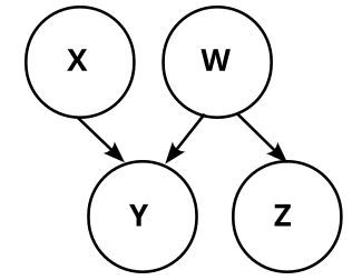
In the causal graph paradigm, we would observe that X and Y are dependent (P(X=0)=10%≠P(X=0|Y=0)=182). Thus we are not able to distinguish between these three causal graphs:
We don’t know whether X causes Y, Y causes X, or there is some common factor W that causes both.
How do we look at this in the Factored Set Paradigm?
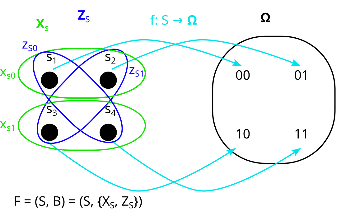
In the factored set paradigm, start with the sample space Ω of our distribution P:
We then say a model of the distribution is a factored set F = (S, B) and a function f:S→Ω:
XS and YS are the “preimages” of X and Y under f. By that I mean that all their parts xSi and ySj are the preimages of xi and yj respectively, under f. That looks as follows:
(Note that in this case f is bijective, but in general f does not have to be bijective. If we allow f to be non-bijective, then the framework works in more generality because we can describe some processes that we couldn’t otherwise describe. [3])
However, we can’t just use any factorization B. In order for (F, f) to count as a model of our distribution P, it needs to be such that the dependencies and independencies of our distribution are represented in the factorization.
That means:
Remember, our probability distribution P was
P(00) = 1%
P(01) = 9%
P(10) = 81%
P(11) = 9%
Is the following actually a model of P?
No, it is not: X, and Y are dependent in P, but XS and YS are orthogonal in F! (Note that orthogonality depends on what model we are in/what factorization we use.)
Here is a really tricky one: Is this a model of P?
Also no, but this is hard to see, so let’s walk through it.
Consider the variable Z = X XOR Y
We don’t have to express our distribution in terms of X and Y, we can just as well define it in terms of X and Z. And then it looks like this:
P(00) = P(X=0, Z=0) = 1%
P(01) = P(X=0, Z=1) = 9%
P(10) = P(X=1, Z=1) = 81%
P(11) = P(X=1, Z=0) = 9%
We can see that Z and X are independent! (becauseP(Z=0)=1%+9%=10%, and alsoP(Z=0|X=0)=1%9%+1%=10% , andP(Z=0|X=1)=9%81%+9%=10%)
What does this mean for our model? It means that ZS and XS need to be orthogonal.
Are ZS and XS orthogonal in our model? Here it is again:
No, because the history for both XS and ZS is {V}, so XS and ZS have an overlapping history.
So F = (S, {VS}) is also not a model of P.
Does our distribution P have a model at all?
Yes - here is a model that actually works for P:
Here hF(XS)={XS} and hF(ZS)= {ZS}, and hF(YS) = {XS,ZS}.
This means XS and ZS are orthogonal, which matches our observation that X and Z are independent in P. Also XS and YS are not orthogonal, which matches our observation that X and Y are dependent in P.
It also means that hF(XS)⊊hF(YS), so XS is strictly before YS.
If XS is strictly before YS, then the causal arrow goes from X to Y, so we have found a causal direction! It’s this one:
From what we know so far, this causal direction X→Y only holds for this particular model (F, f), but in fact, you can also prove that X→Y holds for any model of this distribution P.
So, we just inferred causality from observational (as opposed to interventional) data, in a way that Pearl’s causal models wouldn’t have inferred!
Sanity-checking the result in Pearl’s paradigm
I have encountered a lot of skepticism that we can infer the causality X→Y here. So I’m going to switch back to the Pearl paradigm, and explain why X causes Y if our distribution is P, and we can actually infer that from only observational data without needing interventional data.
This section will assume you know how to determine (in-)dependence in probability distributions and in causal graphs. (If you don’t, you can either just believe me, or learn about it here and here).
Again, say X is the first bit, Y is the second bit, and Z = X XOR Y. Here is our distribution again, in table-form:
The (in-)dependencies we can read from this are:
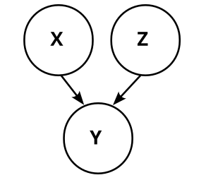
The possible causal graphs which fulfill these dependencies and independencies are these four:
So, we know that Y does not cause X! This matches our finite factored set finding that X causes Y, but it's weaker. Can we also infer that X causes Y?
Let’s concretize the above graphs by adding the conditional probabilities. Graph 1 then looks like this:
Graph 2 is somewhat trickier, because W is not uniquely determined. But one possibility is like this:
Note that W is just the negation of Z here (W=¬Z). Thus, W and Z are information equivalent, and that means graph 2 is actually just graph 1.
Can we find a different variable W such that graph 2 does not reduce to graph 1? I.e. can we find a variable W such that Z is not deterministic given W?
No, we can’t. To see that, consider the distribution P(Z|X,Y,W). By definition of Z, we know that
P(Z|X,Y,W)={1if Z=X XOR Y,0otherwise..
In other words, P(Z|X,Y,W) is deterministic.
We also know that W d-separates Z from X,Y in graph 2:
This d-separation implies that Z is independent from X, Z given W:
P(Z|W)=P(Z|W,X,Y)
As P(Z|X,Y,W) is deterministic, P(Z|W) also has to be deterministic.
So, graph 2 always reduces to graph 1, no matter how we choose W. Analogously, graph 3 and graph 4 also reduce to graph 1, and we know that our causal structure is graph 1:
Which means we also know that X causes Y.
The reason why we usually wouldn’t have found this causal direction using causal graphs is that we wouldn’t even have considered Z as potentially interesting. This is what factored sets give us: They make us consider every possible way of defining variables, so we don’t miss out on any information that may be hidden if we just look at a predetermined set of variables.
Summary
Set factorizations are a way of expressing sets as a product of some factors, similar to how integer factorization is about expressing integers as a product of some factors.
We can define a history on them, that tells us which properties came “before” other properties. We say that two variables are orthogonal if they have no shared history. Using these notions of history and orthogonality, we can define a mathematical structure called model of a probability distribution. With this model, we can do causal inference (inferring causal structure from data).
Factored sets let us infer causal relations that we usually wouldn’t have found using causal graphs. For example, if we have two binary variables X and Y, and X is independent from X XOR Y, then we can infer the causal direction X→Y.
Further Reading
I hope you got a bit of a grasp on finite factored sets, and see why they are really neat. If you want to read more, the best entry point is probably this edited transcript from a talk by Scott Garrabrant.
For a non-mathematical intuition how Scott relates the concepts of time, causality, abstraction, and agency, see his Saving Time post.
I haven’t looked closely into AI alignment specific applications of factored sets, but it looks like they can be used to better talk about embedded agency, decision theory, and ELK.
_____
This post is a result of a distillation workshop led by John Wentworth at SERI MATS. I’d like to thank Leon Lang, Scott Garrabrant, Matt MacDermott, Jesse Hoogland, and Marius Hobbhahn for feedback and discussions on this post.
Note that the number of set factorizations of an n-element set is not the same as the number of integer factorizations of n, because elements are distinguishable, so for example these two factorizations do not count as the same factorization:
Actually, it’s somewhat more complicated than “X and Y are (conditionally) orthogonal if and only if they are independent”. The full version is more like “If XS and YS are partitions on a set S, which has a mapping f:S→Ω to the sample space, then XS and YS are (conditionally) orthogonal if and only if the images X and Y of XS and YS are (conditionally) independent”. But for the sake of this explanation, if you just remember that “orthogonality ⇔ independence”, that's enough.
Even if f is not bijective, the “preimages” XS and YS of X and Y are always well-defined partitions. Here are two examples in which f is not bijective: