Recently, in a group chat with friends, someone posted this Lesswrong post and quoted:

The group consensus on somebody's attractiveness accounted for roughly 60% of the variance in people's perceptions of the person's relative attractiveness.

I answered that, embarrassingly, even after reading Spencer Greenberg's tweets for years, I don't actually know what it means when one says:

$X$ explains $p$ of the variance in $Y$.^[1] 

What followed was a vigorous discussion about the correct definition, and several links to external sources like Wikipedia. Sadly, it seems to me that all online explanations (e.g. on Wikipedia here and here), while precise, seem philosophically wrong since they confuse the platonic concept of explained variance with the variance explained by a statistical model like linear regression. 

The goal of this post is to give a conceptually satisfying definition of explained variance. The post also explains how to approximate this concept, and contains many examples. I hope that after reading this post, you will remember the meaning of explained variance forever.

Audience: Anyone who has some familiarity with concepts like expected values and variance and ideally also an intuitive understanding of explained variance itself. I will repeat the definitions of all concepts, but it is likely easier to appreciate the post if one encountered them before.

Epistemic status: I thought up the "platonically correct" definition I give in this post myself, and I guess that there are probably texts out there that state precisely this definition. But I didn't read any such texts, and as such, there's a good chance that many people would disagree with parts of this post or its framing. Also, note that all plots are fake data generated by Gemini and ChatGPT --- please forgive me for inconsistencies in the details. 

Acknowledgments: Thanks to Tom Lieberum and Niels Doehring for pointing me toward the definition of explained variance that made it into this post. Thank you to Markus Over for giving feedback on drafts. Thanks to ChatGPT and Gemini for help with the figures and some math. 

Definitions

The verbal definition

Assume you observe data like this fake (and unrealistic) height-weight scatterplot of 1000 people:

Let $X$ be the height and $Y$ be the weight of people. Clearly, height is somewhat predictive of weight, but how much? One answer is to look at the extent to which knowledge of $X$ narrows down the space of possibilities for $Y$. For example, compare the spread in weights $Y$ for the whole dataset with the spread for the specific height of 170cm:

The spread in these two curves is roughly what one calls their "variance". That height explains $p$ of the variance in weight then means the following: the spread of weight for a specific height is $1-p$ times the total spread. It's a measure of the degree to which height determines weight! 

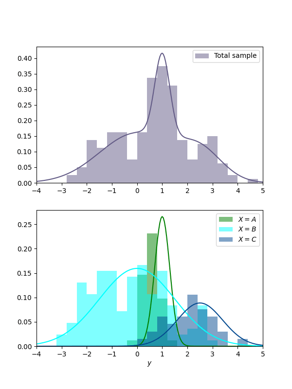
There is a caveat, which is that the spread might differ between different heights. E.g., look at yet another artificial scatter plot:

Here are three projections of the data on $Y$, for small, large, and all values of $X$:

The spread varies massively between different $X$! So which spread do we compare the total spread (blue) with, when making a statement like "$X$ explains $p$ of the variance in $Y$"? The answer is to build the average of the spreads over all values of $X$, weighted by how likely these values of $X$ are. 

Thus, we can translate the sentence

$X$ explains $p$ of the variance in $Y$

to the following verbal definition:

On average, over all different values of $X$ weighted by their probability, the remaining variance in $Y$ is $1-p$ times the total variance in $Y$. 

This is the definition that we will translate to formal math below!

The mathematical definition

We now present a mathematical definition that precisely mirrors the verbal definition above. It's important to understand that the verbal definition is much more general than the figures I presented might suggest. In particular:

• The definition does not presuppose any particular relationship between $X$ and $Y$, like being linear up to some noise.
• The definition does not assume that $X$ and $Y$ live "in the same space". It could be that samples $x$ of $X$ are very complex object, like "all genetic information about a human". But we assume $Y$ to always be representable on a scale.
• The definition does not assume a specific way of predicting $Y$ from $X$. We will come to that later, when talking about regression, which leads to the more widely-used definitions in the literature. 

With that out of the way, recall that we want to translate this sentence to formal math:

On average, over all different values of $X$ weighted by their probability, the remaining variance in $Y$ is $1-p$ times the total variance in $Y$. 

To accomplish this, we model $X$ and $Y$ as random variables, which are jointly sampled according to a density $p(x,y)$. To be fully general, $x$ takes values in some arbitrary (suitable, measurable) space $X$, and $y$ takes values in the real numbers $Y=R$. In regions of the "plane" $X\times R$ where $p(x,y)$ is large, we are more likely to sample datapoints than elsewhere. We can then express the sentence above in the following formula:

We need to explain all the symbols here! Let's start with the total variance in $Y$, which we denote by ${\text{Var}}_{\text{tot}}\left(Y\right)$. It is the average of the squared distance of samples of $Y$ from the mean of $Y$. As a formula:

Note that $p\left(y\right)$ is the marginal density of $y$, which is given from the joint density $p(x,y)$ by $p\left(y\right)={\int }_{x\in X}p(x,y).$ The mean $\mu \left(Y\right)$ that appears in the variance is itself an average, namely over all of $Y$:

What about the average remaining variance, which we denoted $\text{E}[{\text{Var}}_{\text{rem}}(Y\mid X)]$? According to the verbal definition, it is an average of the remaining variances for different values of $x\in X$, weighted by their probability. So we get:

Now we need to explain the inner remaining variance. The idea: It is given in the same way as the total variance of $Y$, except that $y\in R$ is now sampled conditional on $X=x$ being fixed. We obtain:

where $p(y\mid x)=p(x,y)/p\left(x\right)$ is the conditional density, and where the conditional mean is given by

This explains the entire definition! 

If we now want to make a claim of the form "$X$ explains $p$ of the variance of $Y$" and want to determine the fraction of unexplained variance $1-p$ for it, then we simply rearrange the top formula:

The fraction of explained variance is then 

How to approximate $1-p$

I now discuss how to approximate the fraction of unexplained variance $1-p$ via the formula above.

When you have lots of data

Imagine you sample lots of datapoints $(x_1,y_1),\dots ,(x_N,y_N)$, which we conceptually think of as being sampled from the joint distribution $p(x,y)$. Define $\overline{y}$ as the sample mean of $Y$, which approximates the true mean $\mu \left(Y\right)$:

Then we easily get an approximation of the total variance as:

For each $i=1,\dots ,n$, define ${\hat{y}}_i$ as the sample mean of $Y$ taken over all $y_j$ for which $x_j=x_i$. This approximates $\mu (Y\mid X=x_i)$. With $N_i$ the number of $j$ for which $x_j=x_i$, we obtain:

Using the chain rule $p(x,y)=p\left(x\right)p(y\mid x)$, we can approximate the remaining variance as follows:

Putting it together, we obtain:

where the $N$ was canceled in the last step. 

When you have less data: Regression

The formula above is nice in that it converges to the true fraction of unexplained variance when you have lots of data. However, it has the drawback that, unless we have enormous amounts of data, the means ${\hat{y}}_i$ will probably be very inaccurate --- after all, if the specific value $x_i$ appears only once in the data (which is virtually guaranteed if $X$ is itself a continuous random variable in the special case $X=R$), then ${\hat{y}}_i$ is only based on one data point, leading to $y_i={\hat{y}}_i$. The numerator in the fraction then disappears. This results in a very severe case of overfitting in which it falsely "appears" as if $X$ explains all the variance in $Y$: We obtain the estimate $1-p=0$.

This is why in practice the concept is often defined relative to a regression model. Assume that we fit a regression function $f:X\to Y=R$ that approximates the conditional mean of $Y$:

$f\left(x\right)$ represents the best guess for the value of $y$, given that $x$ is known. $f$ can be any parameterized function, e.g. a neural network, that generalizes well. If $X=R$, then $f$ could be given by the best linear fit, i.e. a linear regression. Then, simply define ${\hat{y}}_i:=f\left(x_i\right)$, leading to outwardly the same formula as before:

Here, $1-p$ is the approximate fraction of variance in $Y$ that cannot be explained by the regression model $f$ from $X$. This is precisely the definition in the Wikipedia article on the fraction of variance unexplained.

As far as I can tell, the fraction of variance explained/unexplained is in the literature predominantly discussed relative to a regression model. But I find it useful to keep in mind that there is a platonic ideal that expresses how much variance in $Y$ is truly explained by $X$. We then usually approximate this upon settling on a hopefully well-generalizing statistical model that is as good as possible at predicting $Y$ given knowledge of $X$.

Examples 

We now look at two more examples to make the concept as clear as possible. In the first, we study the variance explained by three different regression models/fits. In the second one, we look at variance explained by genetic information in twin studies, which does not involve any regression (and not even knowledge of the genes in the samples!).

Dependence on the regression model

Assume $X$ is the sidelength of a cube of water and $Y$ is a measurement of its volume. The plot might look something like this:

Up to some noise, the true relationship is $Y\approx X^3$. If you use $h\left(x\right)=x^3$ as our regression fit (green line in the graph), then we explain almost all variance in volume. Consequently, the fraction of variance unexplained by the regression function $h$ is roughly $1-p\approx 0$.

If you do linear regression, then your best fit will look roughly like the blue line, given by $g\left(x\right)=90x-200$. This time, substantial variance remains since the blue line does mostly not go through the actual data points. But we still reduced the total variance substantially since the blue line is on average much closer to the datapoints than the mean over all datapoints is to those points (said mean is approximately $250$). Thus, the fraction of variance unexplained by the regression function $g\left(x\right)$ is somewhere strictly between $0$ and $1$: $0\ll 1-p\ll 1$.

If you do linear regression, but your linear fit is very bad, like $f\left(x\right)=1200$ (red dotted line), then you're so far away from the data that it would have been better to predict the data by their total mean. Consequently, the remaining variance is greater than the total variance and the fraction of variance unexplained is $1-p>1$.^[2]

When you have incomplete data: Twin studies

Now, imagine you want to figure out to what extent genes, $X$, explain the variance in the IQ, $Y$. Also, imagine that it is difficult to make precise gene measurements. How would you go about determining the fraction of unexplained variance $1-p$ in this case? The key obstacle is that all you can measure is IQ values $y_i$, and you don't know the genes $x_i$ of those people. Thus, we cannot determine a regression function $f$, and thus also no estimate ${\hat{y}}_i=f\left(x_i\right)$ to be used in the formula. At first glance this seems like an unsolvable problem; but notice that $x_i$ does not appear in the final formula of $1-p$! If only it was possible to determine an estimate of ${\hat{y}}_i$ ...

There is a rescue, namely twin studies! Assume data $(x_1,y_1),(x_1,y_1^{\prime }),\dots ,(x_N,y_N),(x_N,y_N^{\prime })$ , where $x_i$ are the unknown genes of an identical twin pair, and $(y_i,y_i^{\prime })$ the IQ measures of both twins. We don't use regression but instead use an approach adapted from the true approximation from this section. Define the conditional means by:

Since we only have two datapoints per twin pair, to get an unbiased estimate of the conditional variance $\text{Var}(Y\mid X=x_i)$, we need to multiply the sample variance by a factor of $2$ (we did not need this earlier since we assumed that we have lots of data, or that our regression is well-generalizing).^[3] With this correction, the fraction of unexplained variance computed over all $2N$ datapoints becomes:

Now, notice that^[4]

Consequently, we obtain

This is precisely $1-r$, where $r$ is the intraclass correlation as defined in this wikipedia page. If we apply this formula to a dataset of 32 twin pairs who were separated early in life, then we arrive^[5] at $1-p=0.2059$, meaning that (according to this dataset) genes explain ~79% of the variance in IQ.^[6]

Conclusion

In this post, I explained the sentence "$X$ explains $p$ of the variance in $Y$" as follows:

On average, over all different values of $X$ weighted by their probability, the remaining variance in $Y$ is $1-p$ times the total variance in $Y$. 

If an intuitive understanding of this sentence is all you take away from this post, then this is a success.

I then gave a precise mathematical definition and explained how to approximate the fraction of unexplained variance $1-p$ when you have lots of data --- which then approximates the platonic concept --- and when you don't; in this case, you get the fraction of variance unexplained by a regression function. 

In a first example, I then showed that the fraction of variance explained by a regression function sensitively depends on that function. In a second example, I explained how to use a dataset of twins to determine the fraction of variance in IQ explained by genes. This differs from the other examples in the fact that we don't need to measure genes (the explaining variable $X$) in order to determine the final result. 

1. ^{^}

   In the whole post, $p$ is a number usually between $0$ and $1$.

2. ^{^}

   Yes, this means that the fraction of explained variance is $p<0$: the model is really an anti-explanation. 

3. ^{^}

   Here is a rough intuition for why we need that factor. Assume you have a distribution $p\left(y\right)$ and you sample two datapoints $y,y^{\prime }$ with sample mean $\hat{y}=\frac{y+y^{\prime }}{2}$. The true variance is given by

   $$\text{Var}\left(Y\right)={\int }_{y}p\left(y\right)\cdot (y-\mu \left(Y\right){)}^2.$$

   Note that $\mu \left(Y\right)$ does not depend on $y$! Thus, if we knew $\mu \left(Y\right)$, then the following would be an unbiased estimate of said variance:

   $$1/2\cdot [(y-\mu (Y){)}^2+(y^{\prime }-\mu \left(Y\right){)}^2].$$

   However, we don't know the true mean, and so the sample variance we compute is

   $$1/2\cdot [(y-\hat{y}{)}^2+(y^{\prime }-\hat{y}{)}^2].$$

   Now the issue is roughly that $\hat{y}$ is precisely in the center between $y$ and $y^{\prime }$, which leads to this expression being systematically smaller than with $\hat{y}$ being replaced by $\mu \left(Y\right)$. Mathematically, it turns out that the best way to correct for this bias is to multiply the estimate of the variance by precisely $2$. See the Wikipedia page for details for general sample sizes. 

4. ^{^}

   Thanks to Gemini 2.5 pro for noticing this for me. 

5. ^{^}

   Code written by Gemini.

6. ^{^}

   There are lots of caveats to this. For example, this assumes that twins have the same genetic distribution as the general population, and that the environmental factors influencing their IQ are related to their genes in the same way as for the general population.