The ultimate goal of John Wentworth’s sequence "Basic Foundations for Agent Models" is to prove a selection theorem of the form:
- Premise (as stated by John): “a system steers far-away parts of the world into a relatively-small chunk of their state space”
- Desired conclusion: The system is very likely (probability approaching 1 with increasing model size / optimization power / whatever) consequentialist, in that it has an internal world-model and search process. Note that this is a structural rather than behavioral property.
John has not yet proved such a result and it would be a major advance in the selection theorems agenda. I also find it plausible that someone without specific context could do meaningful work here. As such, I’ll offer a $5000 bounty to anyone who finds a precise theorem statement and beats John to the full proof (or disproof + proof of a well-motivated weaker statement). This bounty will decrease to zero as the sequence is completed and over the next ~12 months. Partial contributions will be rewarded proportionally.
Probably confused noob question:
It seems like your core claim is that we can reinterpret expected-utility maximizers as expected-number-of-bits-needed-to-describe-the-world-using-M2 minimizers, for some appropriately chosen model of the world M2.
If so, then it seems like something weird is happening, because typical utility functions (e.g. "pleasure - pain" or "paperclips") are unbounded above and below, whereas bits are bounded below, meaning a bit-minimizer is like a utility function that's bounded above: there's a best possible state the world could be in according to that bit-minimizer.
Or are we using a version of expected utility theory that says utility must be bounded above and below? (In that case, I might still ask, isn't that in conflict with how number-of-bits is unbounded above?)
The core conceptual argument is: the higher your utility function can go, the bigger the world must be, and so the more bits it must take to describe it in its unoptimized state under M2, and so the more room there is to reduce the number of bits.
If you could only ever build 10 paperclips, then maybe it takes 100 bits to specify the unoptimized world, and 1 bit to specify the optimized world.
If you could build 10^100 paperclips, then the world must be humongous and it takes 10^101 bits to specify the unoptimized world, but still just 1 bit to specify the perfectly optimized world.
If you could build ∞ paperclips, then the world must be infinite, and it takes ∞ bits to specify the unoptimized world. Infinities are technically challenging, and John's comment goes into more detail about how you deal with this sort of case.
For more intuition, notice that exp(x) is a bijective function from (-∞, ∞) to (0, ∞), so it goes from something unbounded on both sides to something unbounded on one side. That's exactly what's happening here, where utility is unbounded on both sides and gets mapped to something that is unbounded only on one side.
Awesome question! I spent about a day chewing on this exact problem.
First, if our variables are drawn from finite sets, then the problem goes away (as long as we don't have actually-infinite utilities). If we can construct everything as limits from finite sets (as is almost always the case), then that limit should involve a sequence of world models.
The more interesting question is what that limit converges to. In general, we may end up with an improper distribution (conceptually, we have to carry around two infinities which cancel each other out). That's fine - improper distributions happen sometimes in Bayesian probability, we usually know how to handle them.
Thanks for the reply, but I might need you to explain/dumb-down a bit more.
--I get how if the variables which describe the world can only take a finite combination of values, then the problem goes away. But this isn't good enough because e.g. "number of paperclips" seems like something that can be arbitrarily big. Even if we suppose they can't get infinitely big (though why suppose that?) we face problems, see below.
--What does it mean in this context to construct everything as limits from finite sets? Specifically, consider someone who is a classical hedonistic utilitarian. It seems that their utility is unbounded above and below, i.e. for any setting of the variables, there is a setting which is a zillion times better and a setting which is a zillion times worse. So how can we interpret them as minimizing the bits needed to describe the variable-settings according to some model M2? For any M2 there will be at least one minimum-bit variable-setting, which contradicts what we said earlier about every variable-setting having something which is worse and something which is better.
I'll answer the second question, and hopefully the first will be answered in the process.
First, note that , so arbitrarily large negative utilities aren't a problem - they get exponentiated, and yield probabilities arbitrarily close to 0. The problem is arbitrarily large positive utilities. In fact, they don't even need to be arbitrarily large, they just need to have an infinite exponential sum; e.g. if is for any whole number of paperclips , then to normalize the probability distribution we need to divide by . The solution to this is to just leave the distribution unnormalized. That's what "improper distribution" means: it's a distribution which can't be normalized, because it sums to .
The main question here seems to be "ok, but what does an improper distribution mean in terms of bits needed to encode X?". Basically, we need infinitely many bits in order to encode X, using this distribution. But it's "not the same infinity" for each X-value - not in the sense of "set of reals is bigger than the set of integers", but in the sense of "we constructed these infinities from a limit so one can be subtracted from the other". Every X value requires infinitely many bits, but one X-value may require 2 bits more than another, or 3 bits less than another, in such a way that all these comparisons are consistent. By leaving the distribution unnormalized, we're effectively picking a "reference point" for our infinity, and then keeping track of how many more or fewer bits each X-value needs, compared to the reference point.
In the case of the paperclip example, we could have a sequence of utilities which each assigns utility to any number of paperclips X < (i.e. 1 util per clip, up to clips), and then we take the limit . Then our unnormalized distribution is , and the normalizing constant is , which grows like as . The number of bits required to encode a particular value is
Key thing to notice: the first term, , is the part which goes to with , and it does not depend on . So, we can take that term to be our "reference point", and measure the number of bits required for any particular relative to that reference point. That's exactly what we're implicitly doing if we don't normalize the distribution: ignoring normalization, we compute the number of bits required to encode X as
... which is exactly the "adjustment" from our reference point.
(Side note: this is exactly how information theory handles continuous distributions. An infinite number of bits is required to encode a real number, so we pull out a term which diverges in the limit , and we measure everything relative to that. Equivalently, we measure the number of bits required to encode up to precision , and as long as the distribution is smooth and is small, the number of bits required to encode the rest of using the distribution won't depend on the value of .)
Does this make sense? Should I give a different example/use more English?
This gives a nice intuitive explanation for the Jeffery-Bolker rotation which basically is a way of interpreting a belief as a utility, and vice versa.
Some thoughts:
- What do probabilities mean without reference to any sort of agent? Presumably it has something to do with the ability to "win" De Finetti games in expectation. For avoiding subtle anthropomorphization, it might be good to think of this sort of probability as being instantiated in a bacterium's chemical sensor, or something like that. And in this setting, it's clear it wouldn't mean anything without the context of the bacterium. Going further, it seems to me like the only mechanism which makes this mean anything is the fact that it helps make the bacterium "exist more" i.e. reproduce and thrive. So I think having a probability mean a probability inherently requires some sort of self-propagation -- it means something if it's part of why it exists. This idea can be taken to an even deeper level, where according to Zureck you can get the Born probabilities by looking at what quantum states allow information to persist through time (from within the system).
- Does this imply anything about the difficulty of value learning? An AGI will be able to make accurate models of the world, so it will have the raw algorithms needed to do value learning... the hard part seems to be, as usual, pointing to the "correct" values. Not sure this helps with that so much.
- A bounded agent creating a model will have to make decisions about how much detail to model various aspects of the world in. Can we use this idea to "factor" out that sort of trade-off as part of the utility function?
I don't see the connection to the Jeffrey-Bolker rotation? There, to get the shouldness coordinate, you need to start with the epistemic probability measure, and multiply it by utility; here, utility is interpreted as a probability distribution without reference to a probability distribution used for beliefs.
I think someone should show what P(X|M_2) looks like after a Jeffrey-Bolker rotation, and see if there's a nice interpretation of what happens.
Summary
I summarize this post in a slightly reverse order. In AI alignment, one core question is how to think about utility maximization. What are agents doing that maximize utility? How does embeddedness play into this? What can we prove about such agents? Which types of systems become maximizers of utility in the first place?
This article reformulates expected utility maximization in equivalent terms in the hopes that the new formulation makes answering such questions easier. Concretely, a utility function u is given, and the goal of a u-maximizer is to change the distribution M1 over world states X in such a way that E_M1[u(X)] is maximized. Now, assuming that the world is finite (an assumption John doesn’t mention but is discussed in the comments), one can find a>0, b such that a*u(X) + b = log P(X | M2) for some distribution/model of the world M2. Roughly, M2 assigns high probability to states X that have high utility u(X).
Then the equivalent goal of the u-maximizer becomes changing M1 such that E_M1[- log P(X | M2)] becomes minimal, which means minimizing H(X | M1) + D_KL(M1 | M2). The entropy H(X | M1) cannot be influenced in our world (due to thermodynamics) or can, by a mathematical trick, be assumed to be fixed, meaning that the problem reduces to just minimizing the KL-distance of distributions D_KL(M1 | M2). Another way of saying this is that we want to minimize the average number of bits required to describe the world state X when using the Shannon-Fano code of M2. A final tangential claim is that for powerful agents/optimization processes, the initial M1 with which the world starts shouldn’t matter so much for the achieved end result of this process.
John then speculates on how this reformulation might be useful, e.g. for selection theorems.
Opinion
This is definitely thought-provoking.
What I find interesting about this formulation is that it seems a bit like “inverse generative modeling”: usually in generative modeling in machine learning, we start out with a “true distribution” M1’ of the world and try to “match” a model distribution M2’ to it. This can then be done by maximizing average log P(X | M2’) for X that are samples from M1’, i.e. by performing maximum likelihood. So in some sense, a “utility” is maximized there as well.
But in John’s post, the situation is reversed: the agent has a utility function corresponding to a distribution M2 that weights up desired world states, and the agent tries to match the real-world distribution M1 to that.
If an agent is now both engaging in generative modeling (to build its world model) and in utility maximization, then it seems like the agent could also collapse both objectives into one: start out with the “wrong” prediction by already assuming the desired world state M2 and then get closer to predicting correctly by changing the real world. Noob question: is this what the predictive processing people are talking about? I’m wondering this since when I heard people saying things like “all humans do is just predicting the world”, I never understood why humans wouldn’t then just sit in a dark room without anything going on, which is a highly predictable world-state. The answer might be that they start out predicting a desirable world, and their prediction algorithm is somehow weak and only manages to predict correctly by “just” changing the world. I’m not sure if I buy this.
One thing I didn’t fully understand in the post itself is why the entropy under M1 can always be assumed to be constant by a mathematical trick, though another comment explored this in more detail (a comment I didn’t read in full).
Minor: Two minus signs are missing in places, and I think the order of the distributions in the KL term is wrong.
Promoted to curated: As Adele says, this feels related to a bunch of the Jeffery-Bolker rotation ideas, which I've referenced many many times since then, but in a way that feels somewhat independent, which makes me more excited about there being some deeper underlying structure here.
I've also had something like this in my mind for a while, but haven't gotten around to formalizing it, and I think I've seen other people make similar arguments in the past, which makes this a valuable clarification and synthesis that I expect to get referenced a bunch.
In my Phd thesis I explored an extension of the compression/modeling equivalence that's motivated by Algorithmic Information Theory. AIT says that if you have a "perfect" model of a data set, then the bitstream created by encoding the data using the model will be completely random. Every statistical test for randomness applied to the bitstream will return the expected value. For example, the proportion of 1s should be 0.5, the proportion of 1s following the prefix 010 should be 0.5, etc etc. Conversely, if you find a "randomness deficiency", you have found a shortcoming of your model. And it turns out you can use this info to create an improved model.
That gives us an alternative conceptual approach to modeling/optimization. Instead of maximizing a log-likelihood, take an initial model, encode the dataset, and then search the resulting bitstream for randomness deficiencies. This is very powerful because there is an infinite number of randomness tests that you can apply. Once you find a randomness deficiency, you can use it to create an improved model, and repeat the process until the bitstream appears completely random.
The key trick that made the idea practical is that you can use "pits" instead of bits. Bits are tricky, because as your model gets better, the number of bits goes down - that's the whole point - so the relationship between bits and the original data samples gets murky. A "pit" is a [0,1) value calculated by applying the Probability Integral Transform to the data samples using the model. The same randomness requirements hold for the pitstream as for the bitstream, and there are always as many pits as data samples. So now you can define randomness tests based on intuitive contexts functions, like "how many pits are in the [0.2,0.4] interval when the previous word in the original text was a noun?"
Interesting framing. Do you have a unified strategy for handling the dimensionality problem with sub-exponentially-large datasets, or is that handled mainly by the initial models (e.g. hidden markov, bigram, etc)?
I'm not sure exactly what you mean, but I'll guess you mean "how do you deal with the problem that there are an infinite number of tests for randomness that you could apply?"
I don't have a principled answer. My practical answer is just to use good intuition and/or taste to define a nice suite of tests, and then let the algorithm find the ones that show the biggest randomness deficiencies. There's probably a better way to do this with differentiable programming - I finished my Phd in 2010, before the deep learning revolution.
Late comment here, but I really liked this post and want to make sure I've fully understood it. In particular there's a claim near the end which says: if is not fixed, then we can build equivalent models , for which it is fixed. I'd like to formalize this claim to make sure I'm 100% clear on what it means. Here's my attempt at doing that:
For any pair of models , where , there exists a variable (of which is a subset) and a pair of models , such that 1) for any , ; and 2) the behavior of the system is the same under , as it was under , .
To satisfy this claim, we construct our as the conjunction of and some "extra" component . e.g., for a coin flip, for a die roll, and so is the conjunction of the coin flip and the die roll, and the domain of is the outer product of the coin flip domain and of the die roll domain.
Then we construct our by imposing 1) (i.e., , are logically independent given for every ); and 2) (i.e., the marginal prob given equals the original prob under ).
Finally we construct by imposing the analogous 2 conditions that we did for : 1) and 2) . But we also impose the extra condition 3) (assuming finite sets, etc.).
We can always find , and that satisfy the above conditions, and with these choices we end up with for all , (i.e., is fixed) and (i.e., the system retains the same dynamics).
Is this basically right? Or is there something I've misunderstood?
The construction is correct.
Note that for , conceptually we don't need to modify it, we just need to use the original but apply it only to the subcomponents of the new -variable which correspond to the original -variable. Alternatively, we can take the approach you do: construct which has a distribution over the new , but "doesn't say anything" about the new components, i.e. the it's just maxentropic over the new components. This is equivalent to ignoring the new components altogether.
Ah yes, that's right. Yeah, I just wanted to make this part fully explicit to confirm my understanding. But I agree it's equivalent to just let ignore the extra (or whatever) component.
Thanks very much!
I'm really excited about this post, as it relates super closely to a recent paper I published (in Science!) about spontaneous organization of complex systems - like when a house builds itself somehow, or utility self-maximizes just following natural dynamics of the world. I have some fear of spamming, but I'm really excited others are thinking along these lines - so I wanted to share a post I wrote explaining the idea in that paper https://medium.com/bs3/designing-environments-to-select-designs-339d59a9a8ce
Would love to hear your thoughts!
Note for others: link to the paper from that post is gated, here's the version on arxiv, though I did not find links to the videos. It is a very fun paper.
Thanks for your interest - really nice to hear! here is a link to the videos (and supplement): https://science.sciencemag.org/content/suppl/2020/12/29/371.6524.90.DC1
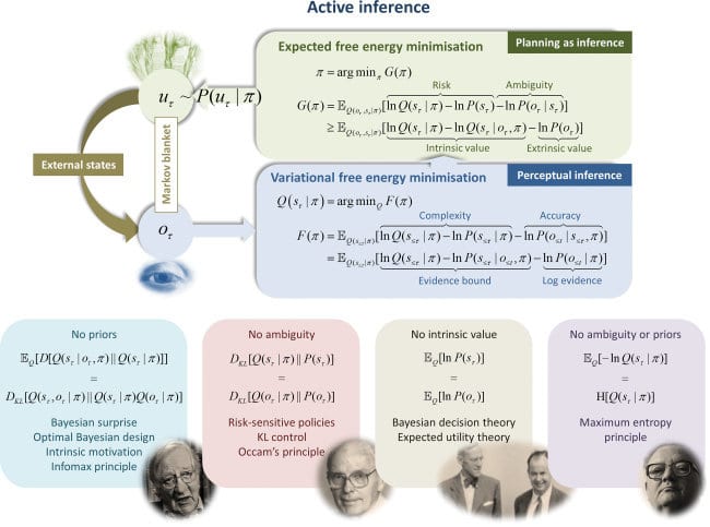
I know you've acknowledged Friston at the end, but I'm just commenting for other interested readers' benefit that this is very close to Karl Friston’s active inference framework, which posits that all agents minimise the discrepancies (or prediction errors) between their internal representations of the world and their incoming sensory information through both action and perception.
It's worth emphasising just how closely related it is. Fristons' expected free energy of a policy is, where the first term is the expected information gained by following the policy and the second the expected 'extrinsic value'.
The extrinsic value term , translated into John's notation and setup, is precisely . Where John has optimisers choosing to minimise the cross-entropy of under with respect to under , Friston has agents choosing to minimise the cross-entropy of preferences () with respect to beliefs ().
What's more, Friston explicitly thinks of the extrinsic value term as a way of writing expected utility (see the image below from one of his talks). In particular is a way of representing real-valued preferences as a probability distribution. He often constucts by writing down a utility function and then taking a softmax (like in this rat T-maze example), which is exactly what John's construction amounts to.
It seems that John is completely right when he speculates that he's rediscovered an idea well-known to Karl Friston.
I have an intuition that this might have implications for the Orthogonality Thesis, but I'm quite unsure. To restate the Orthogonality Thesis in the terms above, "any combination of intelligence level and model of the world, M2". This feels different than my intuition that advanced intelligences will tend to converge upon a shared model / encoding of the world even if they have different goals. Does this make sense? Is there a way to reconcile these intuitions?
Important point: neither of the models in this post are really "the optimizer's model of the world". is an observer's model of the world (or the "God's-eye view"); the world "is being optimized" according to that model, and there isn't even necessarily "an optimizer" involved. says what the world is being-optimized-toward.
To bring "an optimizer" into the picture, we'd probably want to say that there's some subsystem which "chooses"/determines , in such a way that , compared to some other -values. We might also want to require this to work robustly, across a range of environments, although the expectation does that to some extent already. Then the interesting hypothesis is that there's probably a limit to how low such a subsystem can make the expected-description-length without making depend on other variables in the environment. To get past that limit, the subsystem needs things like "knowledge" and a "model" of its own - the basic purpose of knowledge/models for an optimizer is to make the output depend on the environment. And it's that model/knowledge which seems likely to converge on a similar shared model/encoding of the world.
Thanks! I'm still wrapping my mind around a lot of this, but this gives me some new directions to think about.
The title, "Utility Maximization = Description Length Minimization", and likewise the bolded statement, "to “optimize” a system is to reduce the number of bits required to represent the system state using a particular encoding", strike me as wrong in the general case, or as only true in a degenerate sense that can't imply much. This is unfortunate, because it inclines me to dismiss the rest of the post.
Suppose that the state of the world can be represented in 100 bits. Suppose my utility function assigns a 0 to each of 2^98 states (which I "hate"), and a 1 to all the remaining (2^100 - 2^98) states (which I "like"). Let's imagine I chose those 2^98 states randomly, so there is no discernible pattern among them.
You would need 99.58 bits to represent one state out of the states that I like. So "optimizing" the world would mean reducing it from a 100-bit space to a 99.58-bit space (which you would probably end up encoding with 100 bits in practice). While it's technically true that optimizing always implies shrinking the state space, the amount of shrinking can be arbitrarily tiny, and is not necessarily proportional to the amount by which the expected utility changes. Thus my objection to the title and early statement.
It probably is true in practice that most real utility functions are much more constraining than the above scenario. (For example, if you imagine all the possible configurations of the atoms that make up a human, only a tiny fraction of them correspond to a living human.) There might be interesting things to say about that. However, the post doesn't seem to base its central arguments on that.
Given what is said later about using K-L divergence to decompose the problem into "reducing entropy" + "changing between similar-entropy distributions", I could say that the post makes the case for me: that a more accurate title would be "Utility Maximization = Description Length Minimization + Other Changes" (I don't have a good name for the second component).
I actually think this is a feature, not a bug. In your example, you like 3/4 of all possible world states. Satisfying your preferences requires shrinking the world-space by a relatively tiny amount, and that's important. For instance:
- From the perspective of another agent in the universe, satisfying your preferences is very likely to incur very little opportunity cost for the other agent (relevant e.g. when making deals)
- From your own perspective, satisfying your preferences is "easy" and "doesn't require optimizing very much"; you have a very large target to hit.
While it's technically true that optimizing always implies shrinking the state space, the amount of shrinking can be arbitrarily tiny, and is not necessarily proportional to the amount by which the expected utility changes.
Remember that utility functions are defined only up to scaling and shifting. If you multiply a utility function by 0.00001, then it still represents the exact same preferences. There is not any meaningful sense in which utility changes are "large" or "small" in the first place, except compared to other changes in the same utility function.
On the other hand, optimization-as-compression does give us a meaningful sense in which changes are "large" or "small".
There is not any meaningful sense in which utility changes are "large" or "small" in the first place, except compared to other changes in the same utility function.
We can establish a utility scale by tweaking the values a bit. Let's say that in my favored 3/4 of the state space, half the values are 1 and the other half are 2. Then we can set the disfavored 1/4 to 0, to -100, to -10^100, etc., and get utility functions that aren't equivalent. Anyway, in practice I expect we would already have some reasonable unit established by the problem's background—for example, if the payoffs are given in terms of number of lives saved, or in units of "the cost of the action that 'optimizes' the situation".
Satisfying your preferences requires shrinking the world-space by a relatively tiny amount, and that's important. [...] satisfying your preferences is "easy" and "doesn't require optimizing very much"; you have a very large target to hit.
So the theory is that the fraction by which you shrink the state space is proportional (or maybe its logarithm is proportional) to the effort involved. That might be a better heuristic than none at all, but it is by no means true in general. If we say I'm going to type 100 digits, and then I decide what those digits are and type them out, I'm shrinking the state-space by 10^100. If we say my net worth is between $0 and $10^12, and then I make my net worth be $10^12, I'm shrinking the state-space (in that formulation of the world) by only 10^12 (or perhaps 10^14 if cents are allowed); but the former is enormously easier for me to do than the latter. In practice, again, I think the problem's background would give much better ways to estimate the cost of the "optimization" actions.
(Edit: If you want an entirely self-contained example, consider: A wall with 10 rows of 10 cubby-holes, and you have 10 heavy rocks. One person wants the rocks to fill out the bottom row, another wants them to fill out the left column, and a third wants them on the top row. At least if we consider the state space to just be the positions of the rocks, then each of these people wants the same amount of state-space shrinking, but they cost different amounts of physical work to arrange.)
I'm guessing that the best application of the idea would be as one of the basic first lenses you'd use to examine/classify a completely alien utility function.
If you want an entirely self-contained example, consider: A wall with 10 rows of 10 cubby-holes, and you have 10 heavy rocks. One person wants the rocks to fill out the bottom row, another wants them to fill out the left column, and a third wants them on the top row. At least if we consider the state space to just be the positions of the rocks, then each of these people wants the same amount of state-space shrinking, but they cost different amounts of physical work to arrange.)
I think what's really going on in this example (and probably implicitly in your intuitions about this more generally) is that we're implicitly optimizing only one subsystem, and the "resources" (i.e. energy in this case, or money) is what "couples" optimization of this subsystem with optimization of the rest of the world.
Here's what that means in the context of this example. Why is putting rocks on the top row "harder" than on the bottom row? Because it requires more work/energy expenditure. But why does energy matter in the first place? To phrase it more suggestively: why do we care about energy in the first place?
Well, we care about energy because it's a limited and fungible resource. Limited: we only have so much of it. Fungible: we can expend energy to gain utility in many different ways in many different places/subsystems of the world. Putting rocks on the top row expends more energy, and that energy implicitly has an opportunity cost, since we could have used it to increase utility in some other subsystem.
More generally, the coherence theorems typically used to derive expected utility maximization implicitly assume that we have exactly this sort of resource. They use the resource as a "measuring stick"; if a system throws away the resource unnecessarily (i.e. ends up in a state which it could have gotten to with strictly less expenditure of the resource), then the system is suboptimal for any possible utility function for which the resource is limited and fungible.
Tying this all back to optimization-as-compression: we implicitly have an optimization constraint (i.e. the amount of resource) and likely a broader world in which the limited resource can be used. In order for optimization-as-compression to match intuitions on this problem, we need to include those elements. If energy can be expended elsewhere in the world to reduce description length of other subsystems, then there's a similar implicit bit-length cost of placing rocks on the top shelf. (It's conceptually very similar to thermodynamics: energy can be used to increase entropy in any subsystem, and temperature quantifies the entropy-cost of dumping energy into one subsystem rather than another.)
Hmm. If we bring actual thermodynamics into the picture, then I think that energy stored in some very usable way (say, a charged battery) has a small number of possible states, whereas when you expend it, it generally ends up as waste heat that has a lot of possible states. In that case, if someone wants to take a bunch of stored energy and spend it on, say, making a robot rotate a huge die made of rock into a certain orientation, then that actually leads to a larger state space than someone else's preference to keep the energy where it is, even though we'd probably say that the former is costlier than the latter. We could also imagine a third person who prefers to spend the same amount of energy arranging 1000 smaller dice—same "cost", but exponentially (in the mathematical sense) different state space shrinkage.
It seems that, no matter how you conceptualize things, it's fairly easy to construct a set of examples in which state space shrinkage bears little if any correlation to either "expected utility" or "cost".
Potentially challenging example: let's say there's a server that's bottlenecked on some poorly optimized algorithm, and you optimize it to be less redundant, freeing resources that immediately gets used for a wide range of unknown but presumably good tasks.
Superficially, this seems like an optimization that increased the description length. I believe the way this is solved in the OP is that the distributions are constructed in order to assign an extra long description length to undesirable states, even if these undesirable states are naturally simpler and more homogenous than the desirable ones.
I am quite suspicious that this risks you end up with improper probability distributions. Maybe that's OK.
Note that the "thing which is compressed" is the optimization target, which is not the whole system. So in your example, it probably wouldn't be the code itself which is compressed, but rather the runtime of the program (holding the output constant), or maybe the runtimes of a bunch of programs on the machine, or something along those lines.
(Not sure if by "runtime" you mean "time spent running" or "memory/program state during the running time" (or something else)? I was imagining memory/program state in mine, though that is arguably a simplification since the ultimate goal is probably something to do with the business.)
What is the exact formal difference/relation between probability distribution , random variable , and causal model ?
Good question. I recommend looking at this post. The very short version is:
- isn't itself a distribution. It's an operator which takes in a model (i.e. ), and spits out distributions of events/variables defined in that model (i.e. ).
- The model contains some random variables (i.e. and maybe others), and somehow specifies how to sample them. I usually picture as either a Judea Pearl-style causal DAG, or a program which calls rand() sometimes.
- is a variable in the model.
If were so general that by judicious choice of you could impose an arbitrary distribution on then you'd pick the distribution that has , where . That is, a distribution where .
For me, that detracts a little from the entropy + KL divergence decomposition as applied to your utility maximisation problem. No balance point is reached; it's all about the entropy term. Contrast with the bias/variance trade-off (which has applicability to the reference class problem), where balance between the two parts of the decomposition is very important.
It's not quite all about the entropy term; it's the KL-div term that determines which value is chosen. But you are correct insofar as this is not intended to be analogous to bias/variance tradeoff, and it's not really about "finding a balance point" between the two terms.
Hypothesis: in a predictive coding model, the bottom up processing is doing lossless compression and the top down processing is doing lossy compression. I feel excited about viewing more cognitive architecture problems through a lens of separating these steps.
In the thermodynamic view, utility is the negative of energy, so that pressure points from low utility to high utility.
If dP/dV = u''(x) > 0, then the better off you are, the more you want to move further on the margin (increasing returns) - you're 'insatiable'. If dP/dV = u''(x) < 0, then the better off you are, the less you want to move further on the margin (decreasing returns) - you're 'satiable'.
The Arrow-Pratt absolute risk aversion -u''(x)/u'(x) is commonly used as a measure of risk aversion. In these terms, this is -dP/dV / P = -d/dV ln P (I may have screwed up a minus sign, so just imagine whatever sign makes it work). If we define the bulk modulus K = - V dP/dV as in thermodynamics, then we get that the risk aversion is K/PV. PV is what the total utility would be if the marginal utility was always equal to what it is at the current configuration.
An ideal gas satisfies PV = nRT, or in other words P = T/V (dropping constants). If you integrate at constant temperature, then you get Work = T ln V (up to reference points and whatever). That is, an ideal gas is like an agent with log utility.
You could probably continue this "thermodynamics of utility".
The Jeffrey-Bolker rotation is like converting to a risk-neutral measure: we become more risk liking at the expense of making bad outcomes more likely. So, the true distribution assigns more weight to bad outcomes, while our "rosy" model M_2 is more conservative about the bad outcomes (exponential decay to 1 nat of surprise, instead of -Utility of surprise) and quite hopeful about the good outcomes. So I think you lose less error on the bad outcomes when they happen, but they happen more often; likewise you gain more accuracy on the good outcomes when they happen, but they happen less often, in a way that balances out.
There's a minor error in the formula giving the cross entropy: you need a minus sign on the RHS so that it reads E[- log P[X|M_2] | M_2]
The preceding text is "Of course, we could be wrong about the distribution - we could use a code optimized for a model M2 which is different from the “true” model M1. In this case, the average number of bits used will be"
However, information-theoretic groundings only talk about probability, not about "goals" or "agents" or anything utility-like. Here, we've transformed expected utility maximization into something explicitly information-theoretic and conceptually natural.
This interpretation of model fitting formalizes goal pursuit, and looks well constructed. I like this as a step forward in addressing my concern about terminology of AI researchers.
I imagine that negentropy could serve as a universal "resource", replacing the "dollars" typically used as a measuring stick in coherence theorems.
I like to say that "entropy has trained mutating replicators to pursue goal called 'information about the entropy to counteract it'. This 'information' is us. It is the world model , which happened to be the most helpful in solving our equation for actions , maximizing our ability to counteract entropy." How would we say that in this formalism?
Laws of physics are not perfect model of the world, thus we do science and research, trying to make ourselves into a better model of it. However, neither we nor AIs choose the model to minimize the length of input for - ultimately, it is the world that induces its model into each of us (including computers) and optimizes it, not the other way around. There's that irreducible computational complexity in this world, which we continue to explore, iteratively improving our approximations, which we call our model - laws of physics. If someone makes a paperclip maximizer, it will die because of world's entropy, unless it maximizes for its survival (i.e., instead of making paperclips, it makes various copies of itself and all the non-paperclip components needed for its copies, searching for better ones at survival).
Related reading linking mutual information to best possible classifier:
https://arxiv.org/pdf/1801.04062.pdf
This one talks about estimating KL divergence and Mutual Information using neural networks, but I'm specifically linking it to show y'all Theorem 1,
Theorem 1 (Donsker-Varadhan representation). The KL divergence admits the following dual representation:
This links the mutual information to the best possible regression. But I haven't figured out exactly how to parse / interpret this.
What if I want greebles?
To misuse localdeity's example, suppose I want to build a wall with as many cubbyholes as possible, so that I can store my pigeons in them. In comparison to a blank wall, each hole makes the wall more complex, since there are more ways to arrange holes than to arrange holes (assuming the wall can accommodate arbitrarily many holes).
Then use an encoding which assigns very long codes to smooth walls. You'll need long codes for the greebled walls, since there's such a large number of greeblings, but you can still use even longer codes for smooth walls.
I don't see how to do that, especially given that it's not a matter of meeting some threshold, but rather of maximizing a value that can grow arbitrarily.
Actually, you don't even need the ways-to-arrange argument. Suppose I want to predict/control the value of a particular nonnegative integer (the number of cubbyholes), with monotonically increasing utility, e.g. . Then the encoding length of a given outcome must be longer than the code length for each greater outcome: . However, code lengths must be a nonnegative integer number of code symbols in length, so for any given encoding there are at most shorter code lengths, so the encoding must fail no later than .
This look like a technical statement of the Anna Karenina principle,
All happy families are alike; each unhappy family is unhappy in its own way.
But then the problem becomes finding the right M which maximises your utility function.The optimal solution might be very unintuitive and it may require a long description to be understood. M will not be (in general) a smooth set.
There’s a useful intuitive notion of “optimization” as pushing the world into a small set of states, starting from any of a large number of states. Visually:
Yudkowsky and Flint both have notable formalizations of this “optimization as compression” idea.
This post presents a formalization of optimization-as-compression grounded in information theory. Specifically: to “optimize” a system is to reduce the number of bits required to represent the system state using a particular encoding. In other words, “optimizing” a system means making it compressible (in the information-theoretic sense) by a particular model.
This formalization turns out to be equivalent to expected utility maximization, and allows us to interpret any expected utility maximizer as “trying to make the world look like a particular model”.
Conceptual Example: Building A House
Before diving into the formalism, we’ll walk through a conceptual example, taken directly from Flint’s Ground of Optimization: building a house. Here’s Flint’s diagram:
The key idea here is that there’s a wide variety of initial states (piles of lumber, etc) which all end up in the same target configuration set (finished house). The “perturbation” indicates that the initial state could change to some other state - e.g. someone could move all the lumber ten feet to the left - and we’d still end up with the house.
In terms of information-theoretic compression: we could imagine a model which says there is probably a house. Efficiently encoding samples from this model will mean using shorter bit-strings for world-states with a house, and longer bit-strings for world-states without a house. World-states with piles of lumber will therefore generally require more bits than world-states with a house. By turning the piles of lumber into a house, we reduce the number of bits required to represent the world-state using this particular encoding/model.
If that seems kind of trivial and obvious, then you’ve probably understood the idea; later sections will talk about how it ties into other things. If not, then the next section is probably for you.
Background Concepts From Information Theory
The basic motivating idea of information theory is that we can represent information using fewer bits, on average, if we use shorter representations for states which occur more often. For instance, Morse code uses only a single bit (“.”) to represent the letter “e”, but four bits (“- - . -”) to represent “q”. This creates a strong connection between probabilistic models/distributions and optimal codes: a code which requires minimal average bits for one distribution (e.g. with lots of e’s and few q’s) will not be optimal for another distribution (e.g. with few e’s and lots of q’s).
For any random variable X generated by a probabilistic model M, we can compute the minimum average number of bits required to represent X. This is Shannon’s famous entropy formula
−∑XP[X|M]logP[X|M]
Assuming we’re using an optimal encoding for model M, the number of bits used to encode a particular value x is logP[X=x|M]. (Note that this is sometimes not an integer! Today we have algorithms which encode many samples at once, potentially even from different models/distributions, to achieve asymptotically minimal bit-usage. The “rounding error” only happens once for the whole collection of samples, so as the number of samples grows, the rounding error per sample goes to zero.)
Of course, we could be wrong about the distribution - we could use a code optimized for a model M2 which is different from the “true” model M1. In this case, the average number of bits used will be
−∑XP[X|M1]logP[X|M2]=−E[logP[X|M2]|M1]
In this post, we’ll use a “wrong” model M2 intentionally - not because we believe it will yield short encodings, but because we want to push the world into states with short M2-encodings. The model M2 serves a role analogous to a utility function. Indeed, we’ll see later on that every model M2 is equivalent to a utility function, and vice-versa.
Formal Statement
Here are the variables involved in “optimization”:
An “optimizer” takes in some parameter-values θ, and returns new parameter-values θ′ such that
E[−logP[X|M2]|M1(θ′)]≤E[−logP[X|M2]|M1(θ)]
… with equality if-and-only-if θ already achieves the smallest possible value. In English: we choose θ′ to reduce the average number of bits required to encode a sample from M1(θ′), using a code optimal for M2. This is essentially just our formula from the previous section for the number of bits used to encode a sample from M1 using a code optimal for M2.
Other than the information-theory parts, the main thing to emphasize is that we’re mapping one parameter-value θ to a “more optimal” parameter-value θ′. This should work for many different “initial” θ-values, implying a kind of robustness to changes in θ. (This is roughly the same concept which Flint captured by talking about “perturbations” to the system-state.) In the context of iterative optimizers, our definition corresponds to one step of optimization; we could of course feed θ′ back into the optimizer and repeat. We could even do this without having any distinguished “optimizer” subsystem - e.g. we might just have some dynamical system in which θ is a function of time, and successive values of θt satisfy the inequality condition.
Finally, note that our model M1 is a function of θ. This form is general enough to encompass all the usual decision theories. For instance, under EDT, M1(θ) would be some base model M conditioned on the data θ. Under CDT, M1(θ) would instead be a causal intervention on a base model M, i.e. M1(θ)=do(M,Θ=θ).
Equivalence to Expected Utility Optimization
Obviously our expression E[−logP[X|M2]|M1(θ)] can be expressed as an expected utility: just set u(X)=logP[X|M2]. The slightly more interesting claim is that we can always go the other way: for any utility function u(X), there is a corresponding model M2, such that maximizing expected utility u(X) is equivalent to minimizing expected bits to encode X using M2.
The main trick here is that we can always add a constant to u(X), or multiply u(X) by a positive constant, and it will still “be the same utility” - i.e. an agent with the new utility will always make the same choices as the old. So, we set
αu(X)+β=logP[X|M2]⟹P[X|M2]=eβeαu(X)
… and look for α,β which give us a valid probability distribution (i.e. all probabilities are nonnegative and sum to 1).
Since everything is in an exponent, all our probabilities will be nonnegative for any α,β, so that constraint is trivially satisfied. To make the distribution sum to one, we simply set β=−ln∑Xeαu(X). So, not only can we find a model M2 for any u(X), we actually find a whole family of them - one for each α>0.
(This also reveals a degree of freedom in our original definition: we can always create a new model M′2 with P[X|M′2]=1ZP[X|M2]α without changing the behavior.)
So What Does This Buy Us?
If this formulation is equivalent to expected utility maximization, why view it this way?
Intuitively, this view gives more semantics to our “utility functions”. They have built-in “meanings”; they’re not just preference orderings.
Mathematically, the immediately obvious step for anyone with an information theory background is to write:
E[−logP[X|M2]|M1]=−∑XP[X|M1]logP[X|M1]+P[X|M1]logP[X|M2]P[X|M1]
=H(X|M1)+DKL(M2.X||M1.X)
The expected number of bits required to encode X using M2 is the entropy of X plus the Kullback-Liebler divergence of (distribution of X under model M2) from (distribution of X under model M1). Both of those terms are nonnegative. The first measures “how noisy” X is, the second measures “how close” the distributions are under our two models.
Intuitively, this math says that we can decompose the objective E[−logP[X|M2]|M1] into two pieces:
Combined with the previous section: we can take any expected utility maximization problem, and decompose it into an entropy minimization term plus a “make-the-world-look-like-this-specific-model” term.
This becomes especially interesting in situations where the entropy of X cannot be reduced - e.g. thermodynamics. If the entropy H(X) is fixed, then only the KL-divergence term remains. In this case, we can directly interpret the optimization problem as “make the world-state distribution look like P[X|M2]”. If we started from an expected utility optimization problem, then we derive a model M2 such that optimizing expected utility is equivalent to making the world look as much as possible like M2.
In fact, even when H(X) is not fixed, we can build equivalent models M′1,M′2 for which it is fixed, by adding new variables to X. Suppose, for example, that we can choose between flipping a coin and rolling a die to determine X0. We can change the model so that both the coin flip and the die roll always happen, and we include their outcomes in X. We then choose whether to set X0 equal to the coin flip result or the die roll result, but in either case the entropy of X is the same, since both are included. M′2 simply ignores all the new components added to X (i.e. it implicitly has a uniform distribution on the new components).
So, starting from an expected utility maximization problem, we can transform to an equivalent minimum coded bits problem, and from there to an equivalent minimum KL-divergence problem. We can then interpret the optimization as “choose θ to make M1(θ) as close as possible to M2”, with closeness measured by KL-divergence.
What I Imagine This Might Be Useful For
In general, interpretations of probability grounded in information theory are much more solid than interpretations grounded in coherence theorems. However, information-theoretic groundings only talk about probability, not about "goals" or "agents" or anything utility-like. Here, we've transformed expected utility maximization into something explicitly information-theoretic and conceptually natural. This seems like a potentially-promising step toward better foundations of agency. I imagine there's probably purely-information-theoretic "coherence theorems" to be found.
Another natural direction to take this in is thermodynamic connections, e.g. combining it with a generalized heat engine. I wouldn't be surprised if this also tied in with information-theoretic "coherence theorems" - in particular, I imagine that negentropy could serve as a universal "resource", replacing the "dollars" typically used as a measuring stick in coherence theorems.
Overall, the whole formulation smells like it could provide foundations much more amenable to embedded agency.
Finally, there's probably some nice connection to predictive processing. In all likelihood, Karl Friston has already said all this, but it has yet to be distilled and disseminated to the rest of us.