Produced while being an affiliate at PIBBSS^[1]. The work was done initially with funding from a Lightspeed Grant, and then continued while at PIBBSS. Work done in collaboration with @Paul Riechers, @Lucas Teixeira, @Alexander Gietelink Oldenziel, and Sarah Marzen. Paul was a MATS scholar during some portion of this work. Thanks to Paul, Lucas, Alexander, Sarah, and @Guillaume Corlouer for suggestions on this writeup.

Introduction

What computational structure are we building into LLMs when we train them on next-token prediction? In this post we present evidence that this structure is given by the meta-dynamics of belief updating over hidden states of the data-generating process. We'll explain exactly what this means in the post. We are excited by these results because

• We have a formalism that relates training data to internal structures in LLMs.
• Conceptually, our results mean that LLMs synchronize to their internal world model as they move through the context window. 
• The computation associated with synchronization can be formalized with a framework called Computational Mechanics. In the parlance of Computational Mechanics, we say that LLMs represent the Mixed-State Presentation of the data generating process. 
• The structure of synchronization is, in general, richer than the world model itself. In this sense, LLMs learn more than a world model.
• We have increased hope that Computational Mechanics can be leveraged for interpretability and AI Safety more generally.
• There's just something inherently cool about making a non-trivial prediction - in this case that the transformer will represent a specific fractal structure - and then verifying that the prediction is true. Concretely, we are able to use Computational Mechanics to make an a priori  and specific theoretical prediction about the geometry of residual stream activations (below on the left), and then show that this prediction holds true empirically (below on the right).

Theoretical Framework

In this post we will operationalize training data as being generated by a Hidden Markov Model (HMM)^[2]. An HMM has a set of hidden states and transitions between them. The transitions are labeled with a probability and a token that it emits. Here are some example HMMs and data they generate.

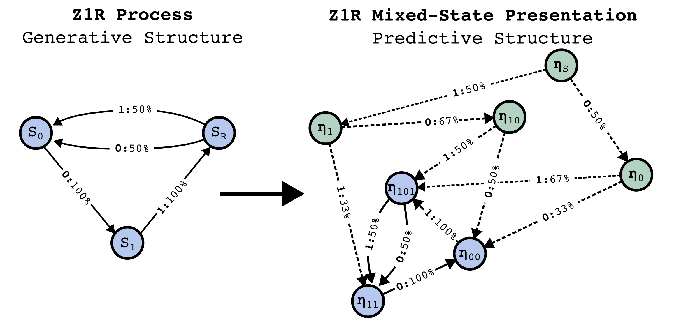
Consider the relation a transformer has to an HMM that produced the data it was trained on. This is general - any dataset consisting of sequences of tokens can be represented as having been generated from an HMM. Through the discussion of the theoretical framework, let's assume a simple HMM with the following structure, which we will call the Z1R process^[3] (for "zero one random"). 

The Z1R process has 3 hidden states, $S_0,S_1,$ and $S_R$. Arrows of the form $S_x\stackrel{\text{a}:p\%}{\to }{S}_y$ denote $P(S_y,\text{a}|S_x)=p\%$, that the probability of moving to state $S_y$ and emitting the token $\text{a}$, given that the process is in state $S_x$, is $p\%$. In this way, taking transitions between the states stochastically generates binary strings of the form ...01R01R... where R is a random 50/50 sample from {0, 1}. 

The HMM structure is not directly given by the data it produces. Think of the difference between the list of strings this HMM emits (along with their probabilities) and the hidden structure itself^[4]. Since the transformer only has access to the strings of emissions from this HMM, and not any information about the hidden states directly, if the transformer learns anything to do with the hidden structure, then it has to do the work of inferring it from the training data. 

What we will show is that when they predict the next token well, transformers are doing even more computational work than inferring the hidden data generating process!

Do Transformers Learn a Model of the World?

One natural intuition would be that the transformer must represent the hidden structure of the data-generating process (ie the "world"^[2]). In this case, this would mean the three hidden states and the transition probabilities between them. 

This intuition often comes up (and is argued about) in discussions about what LLM's "really understand." For instance, Ilya Sutskever has said:

Because if you think about it, what does it mean to predict the next token well enough? It's actually a much deeper question than it seems. Predicting the next token well means that you understand the underlying reality that led to the creation of that token. It's not statistics. Like it is statistics but what is statistics? In order to understand those statistics to compress them, you need to understand what is it about the world that creates this set of statistics.

This type of intuition is natural, but it is not formal. Computational Mechanics is a formalism that was developed in order to study the limits of prediction in chaotic and other hard-to-predict systems, and has since expanded to a deep and rigorous theory of computational structure for any process. One of its many contributions is in providing a rigorous answer to what structures are necessary to perform optimal prediction. Interestingly, Computational Mechanics shows that prediction is substantially more complicated than generation. What this means is that we should expect a transformer trained to predict the next token well should have more structure than the data generating process!

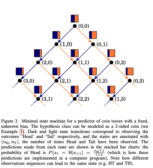
The Structure of Belief State Updating

But what is that structure exactly?

Imagine you know, exactly, the structure of the HMM that produces ...01R... data. You go to sleep, you wake up, and you see that the HMM has emitted a 1. What state is the HMM in now? It is possible to generate a 1 both from taking the deterministic transition  $S_1\stackrel{\text{1}:100\%}{\to }{S}_R$ or from taking  the stochastic transition $S_R\stackrel{\text{1}:50\%}{\to }{S}_0$. Since the deterministic transition is twice as likely as the 50% one, the best you can do is to have some belief distribution over the current states of the HMM, in the case $P\left(\right[S_0,S_1,S_R\left]\right)=[\frac{1}{3},0,\frac{2}{3}]$^[5]. 

If now you see another 1 emitted, so that in total you've seen 11, you can now use your previous belief about the HMM state (read: prior), and your knowledge of the HMM structure alongside the emission you just saw (read: likelihood), in order to generate a new belief state (read: posterior). An exercise for the reader: What is the equation for updating your belief state given a previous belief state, an observed token, and the transition matrix of the ground-truth HMM?^[6] In this case, there is only one way for the HMM to generate 11, $S_1\stackrel{\text{1}:100\%}{\to }{S}_R\stackrel{\text{1}:50\%}{\to }{S}_0$, so you know for certain that the HMM is now in state $S_0$. From now on, whenever you see a new symbol, you will know exactly what state the HMM is in, and we say that you have synchronized to the HMM.

In general, as you observe increasing amounts of data generated from the HMM, you can continually update your belief about the HMM state. Even in this simple example there is non-trivial structure in these belief updates. For instance, it is not always the case that seeing 2 emissions is enough to synchronize to the HMM. If instead of 11... you saw 10... you still wouldn't be synchronized, since there are two different paths through the HMM that generate 10. 

The structure of belief-state updating is given by the Mixed-State Presentation.

The Mixed-State Presentation

Notice that just as the data-generating structure is an HMM - at a given moment the process is in a hidden state, then, given an emission, the process move to another hidden state - so to is your belief updating! You are in some belief state, then given an emission that you observe, you move to some other belief state. 

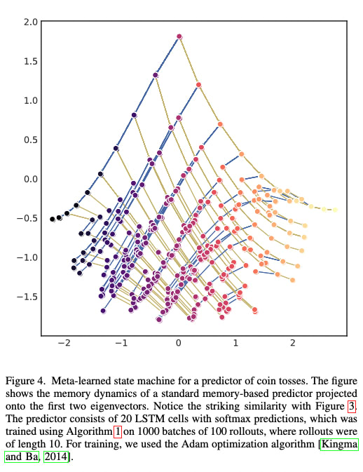
The meta-dynamics of belief state updating are formally another HMM, where the hidden states are your belief states. This meta-structure is called the Mixed-State Presentation (MSP) in Computational Mechanics.

Note that the MSP has transitory states (in green above) that lead to a recurrent set of belief states that are isomorphic to the data-generating process - this always happens, though there might be infinite transitory states. Synchronization is the process of moving through the transitory states towards convergence to the data-generating process.

A lesson from Computational Mechanics is that in order to perform optimal prediction of the next token based on observing a finite-length history of tokens, one must implement the Mixed-State Presentation (MSP). That is to say, to predict the next token well one should know what state the data-generating process is in as best as possible, and to know what state the data-generating process is in, implement the MSP.

The MSP has a geometry associated with it, given by plotting the belief-state values on a simplex. In general, if our data generating process has N states, then probability distributions over those states will have $N-1$ degrees of freedom, and since all probabilities must be between 0 and 1, all possible belief distributions lie on an $N-1$ simplex. In the case of Z1R, that means a 2-simplex (i.e. a triangle). We can plot each of our possible belief states in this 2-simplex, as shown on the right below.

What we show in this post is that when we train a transformer to do next token prediction on data generated from the 3-state HMM, we can find a linear representation of the MSP geometry in the residual stream. This is surprising! Note that the points on the simplex, the belief states, are not the next token probabilities. In fact, multiple points here have literally the same next token predictions. In particular, in this case, ${\eta }_{10}$, ${\eta }_S$, and ${\eta }_{101}$, all have the same optimal next token predictions.

Another way to think about this claim is that transformers keep track of distinctions in anticipated distribution over the entire future, beyond distinctions in next token predictions, even though the transformer is only trained explicitly on next token prediction!  That means the transformer is keeping track of extra information than what is necessary just for the local next token prediction.

Another way to think about our claim is that transformers perform two types of inference: one to infer the structure of the data-generating process, and another meta-inference to update it's internal beliefs over which state the data-generating process is in, given some history of finite data (ie the context window).  This second type of inference can be thought of as the algorithmic or computational structure of synchronizing to the hidden structure of the data-generating process.

A final theoretical note about Computational Mechanics and the theory presented here: because Computational Mechanics is not contingent on the specifics of transformer architectures and is a well-developed first-principles framework, we can apply this framework to any optimal predictor, not just transformers^[7].

Experiment and Results

Experimental Design

To repeat the question we are trying to answer: 

What computational structure are we building into LLMs when we train them on next-token prediction?

To test our theoretical predictions, we designed an experiment with the following steps:

1. Generate training data from a known HMM structure, specifically the 3-state HMM described in the  "Data-Generating Process and MSP" section below.
2. Train a transformer on this data to perform next-token prediction. In the experiments shown here we use a 4-layer transformer with 64 dimensional residual stream, and 4 attention heads per layer.
3. Analyze the final layer of the transformer's residual stream to look for a linear subspace with a geometry matching the predicted fractal structure of the Mixed-State Presentation (MSP).

By controlling the structure of the training data using an HMM, we can make concrete, falsifiable predictions about the computational structure the transformer should implement during inference. Computational Mechanics, as presented in the "Theoretical Framework" section above, provides the framework for making these predictions based on the HMM's structure.

The specific HMM we chose has an MSP with an infinite fractal geometry, serving as a highly non-trivial prediction about what we should find in the transformer's residual stream activations if our theory is correct.

The Data-Generating Process and MSP

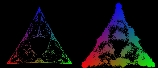
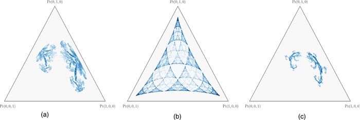
For this experiment we trained a transformer on data generated by a simple HMM, called the Mess3 Process, that has just 3 hidden states^[8]. Moving between the 3 hidden states according to the emission probabilities on the edges generates strings over a 3-token vocabulary: {A, B, C}. The HMM for this data-generating process is given on the left of the figure below.

Our approach allows us to make rigorous and testable predictions about the internal structures of transformers. In the case of this HMM, the theory (outlined above) says that transformers trained on this data should instantiate the computational structure associated with the fractal geometry shown on the right of the figure above. Every colored point in the simplex on the above right panel is a distinct belief state.

We chose the Mess3 HMM because it's MSP has an infinite fractal structure, and thus acts as a highly-nontrivial prediction about what geometry we should find in the residual stream.

The Results!

We train a transformer on data generated by the Mess3 HMM. We look in the final layer of the residual stream and find a linear 2D subspace where activations have a structure remarkably similar to that of our predicted fractal. We do this by performing standard linear regression from the residual stream activations (64 dimensional vectors) to the belief distributions (3 dimensional vectors) which associated with them in the MSP.

We can also look at how this structure emerges over training, which shows (1) that the structure we find is not trivial^[9] since it doesn’t exist in detail early in training, and (2) the step-wise refinement of the transformers activations to the fractal structure we predict. 

A movie of this process is shown below. Because we used Stochastic Gradient Descent for training, the 2D projection of the activations wiggles, even after training has converged. In this wiggling you can see that fractal structures remain intact.

Limitations and Next Steps

Limitations

• Presented here was one simple data structure given by an HMM with 3 states, with a vocab size of 3. In practice, the LLMs that currently exist are much larger, have vocab sizes of >50,000, and natural language has infinite Markov order. Though we've tested this theory on other HMMs and everything continues to work, all tests so far have been on similarly small examples. How this relates to larger, more complicated, and more realistic settings is unknown (but we have ideas!). 
• Though we haven't focused on it in this post, the MSP is an input-driven dynamical system. For each possible input in the system, we have dynamics that determine where in the belief simplex one should move to given the current belief. We have not explicitly tested that the LLM instantiates these dynamics, and instead have only tested that the belief states and their geometry is represented in the transformer.
• Computational Mechanics is primarily a story about optimal prediction. LLMs in practice won't be literally optimal. A number of papers exist studying near-optimality, non-optimality, and rate-distortion phenomenon from the point of view of Computational Mechanics, but applying that to LLMs has not been done.
• We have focused on ergodic and stationary processes in the work presented here. Computational Mechanics can relax those assumptions, but again, we have not applied those (very interesting!) extensions of Computational Mechanics to LLMs. Non-ergodicity, in particular, is likely at the heart of in-context learning.
• In the experiment presented in this post we focussed on the final layer of the residual stream, right before the unembedding. In other experiments we've run (not presented here), the MSP is not well-represented in the final layer but is instead spread out amongst earlier layers. We think this occurs because in general there are groups of belief states that are degenerate in the sense that they have the same next-token distribution. In that case, the formalism presented in this post says that even though the distinction between those states must be represented in the transformers internal, the transformer is able to lose those distinctions for the purpose of predicting the next token (in the local sense), which occurs most directly right before the unembedding.

Next Steps

• We are hopeful that the framing presented in this post provides a formal handle on data structure, internal network structure, and network behavior. 
• There are many open questions about how this work relates to other technical AI Safety work. I'll list a few ideas very quickly, and expand on these and more in future posts. In particular:
  • What is the relationship between features and circuits, as studied in Mechanistic Interpretability, and the Mixed-State Geometry?
  • Is there a story about superposition and compression of the MSP in cases where the residual stream is too small to "fit" the MSP.
  • Can we relate the development of MSP geometric structure over training to phenomenon in SLT? see Towards Developmental Interpretability 
  • Can we use our formalism to operationalize particular capabilities (in-context learning, out-of-distribution generalization, situational awareness, sleeper agents, etc.) and study them in toy models from our framework?
  • Can we use our formalism to understand task structure and how distinct tasks relate to each other? see A starting point for making sense of task structure (in machine learning) 
• As mentioned in the Limitations section, how MSP structures in transformers divide across the layers of the transformer, and how the functional form of the attention mechanism relates to that is an obvious next step.
• We will be releasing a python library soon to be able to perform these types of experiments. Here is the github repo.
• Computational Mechanics is a well-developed framework, and this post has only focused on one small section of it. In the future we hope to bring other aspects of it to bear on neural networks and safety issues, and also to expand Computational Mechanics and combine it with other methods and frameworks. 
• If you're interested in learning more about Computational Mechanics, we recommend starting with these papers: Shalizi and Crutchfield (2000), Riechers and Crutchfield (2018a), and Riechers and Crutchfield (2018b)
• We (Paul and Adam) have received funding to start a new AI Safety research org, called Simplex! Presented here was one small facet of the type of work we hope to do, and very much only the beginning. Stay tuned for posts that outline our broader vision in the future.
• In about a month we will be teaming up with Apart to run a Hackathon! We will post about that soon as well, alongside an open problems post, and some more resources to run experiments.
• There's a lot of work to do going forward! This research plan has many parts that span the highly mathematical/theoretical to experimental. If you are interested in being a part of this please have a low threshold for reaching out! 

1. ^{^}

   PIBBSS is hiring! I wholeheartedly recommend them as an organization. 

2. ^{^}

   One way to conceptualize this is to think of "the world" as having some hidden structure (initially unknown to you), that emits observables. Our task is then to take sequences of observables and infer the hidden structure of the world - maybe in the service of optimal future prediction, but also maybe just because figuring out how the world works is inherently interesting. Inside of us, we have a "world model" that serves as the internal structure that let's us "understand" the hidden structure of the world. The term world model is contentious and nothing in this post depends on that concept much. However, one motivation for this work is to formalize and make concrete statements about peoples intuitions and arguments regarding neural networks and world models - which are often handwavy and ill-defined.

3. ^{^}

   Technically speaking, the term process refers to a probability distribution over infinite strings of tokens, while a presentation refers to a particular HMM that produces strings according to the probability distribution. A process has an infinite number of presentations.

4. ^{^}

   Any HMM defines a probability distribution over infinite sequences of the emissions.

5. ^{^}

   Our initial belief distribution, in this particular case, is the uniform distribution over the 3 states of the data generating process. However this is not always the case. In general the initial belief distribution is given by the stationary distribution of the data generating HMM.

6. ^{^}

   You can find the answer in section IV of this paper by @Paul Riechers.

7. ^{^}

   There is work in Computational Mechanics that studies non-optimal or near-optimal prediction, and the tradeoffs one incurs when relaxing optimality. This is likely relevant to neural networks in practice. See Marzen and Crutchfield 2021 and Marzen and Crutchfield 2014.

8. ^{^}

   This process is called the mess3 process, and was defined in a paper by Sarah Marzen and James Crutchfield. In the work presented we use  x=0.05, alpha=0.85. 

9. ^{^}

   We've also run another control where we retain the ground truth fractal structure but shuffle which inputs corresponds to which points in the simplex (you can think of this as shuffling the colors in the ground truth plot). In this case when we run our regression we get that every residual stream activation is mapped to the center point of the simplex, which is the center of mass of all the points.